
SUM Functions in Excel
The BODMAS formula plays a vital role in the concept of mathematics. BODMAS rule follows the Bracket of Division, Multiplication, Addition and Subtraction. This rule is followed for a correct result, from simple to complex calculations. While doing the calculations manually, the rule is followed, but what if it is done in Excel?
Let’s have a look at the methods in the following steps.
What are Sum Functions in Excel?
The manual calculation takes time and sometimes leads to errors. One can derive a perfect result in Automatic calculations using required formulas. Excel provides default functions for mathematical calculations. Coming to the concept of addition, small numbers are easily added, but what if doing large calculations? Hence using a formula is an effective solution. As excel is widely used for wide applications, it provides default functions for mathematical calculations.
Here in this tutorial, let’s discuss using various Sum formulas in Excel.
1. How to use Sum Formula for adding certain range of cells?
To add the certain range of data in a cell, steps to be followed are,
Step 1: Enter the range of data in the cell.
Step 2: Select the cell where the result wants to display, and type the formula as =SUM(cell range). Here the cell range is mentioned as =SUM(A1:A10)
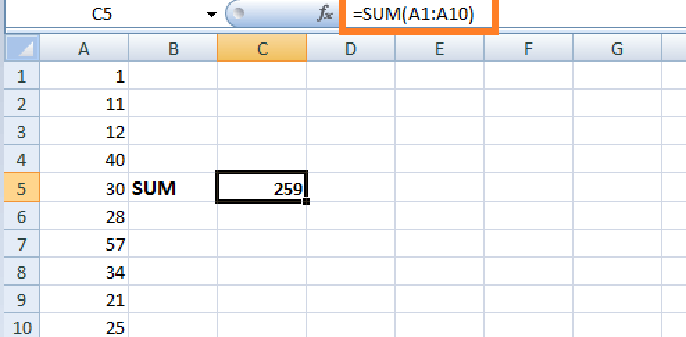
From the above worksheet, the result is displayed as 259 using formula.
2. How to Sum the entire column using Formula?
In certain calculations, the users are supposed to sum the entire column. In such cases, the formulas are used to calculate the entire column.
Step 1: Enter the data in the spreadsheet.
Step 2: Select the cell to display the result and enter the formula as =SUM(A:A) where ‘A’ is the specified cell range. It varies according to user’s preference.
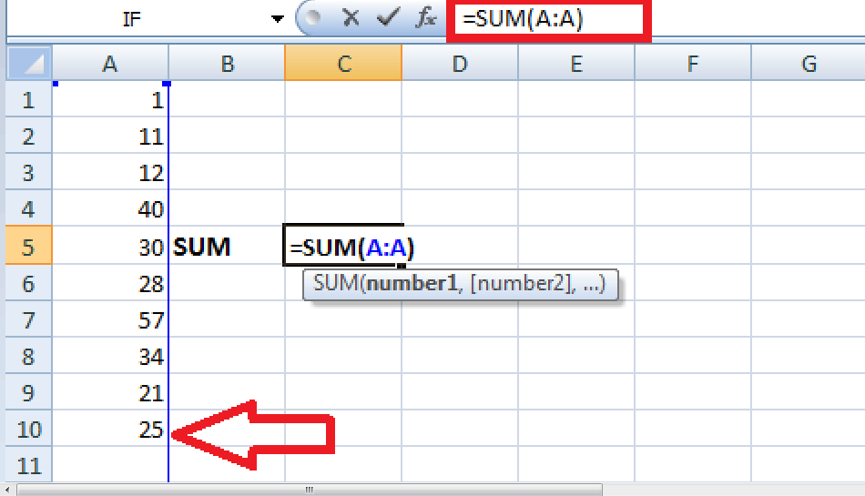
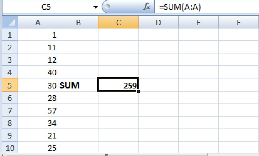
From the above excel chart, when the formula is entered, the blue line selects the entire column of A. The result for entire column is displayed as shown below.
3. How to sum the entire row using Formula?
To calculate the entire row, following methods are used.
Step 1: Enter the data in the spreadsheet.
Step 2: Select the cell to display the result and enter the formula as =SUM(3:3) where ‘3:3’ is the specified row range. It varies according to user’s preference.

Here in the above worksheet, the sum of entire fifth row is calculated and the result is displayed as 30.
4. How to sum non – contagious cell?
Sometimes, in calculations the cell needs to be added for calculations. The cells are added without regular intervals which are not next to each other. This is called non- contagious cell. Formulas used to sum the non-contagious cell are,
=SUM(Specified cell name)
Step1: Enter the data in the spreadsheet.
Step 2: Select the cell where you want to display the result. Enter the formula as =SUM (A2,A4,A6,A8,A10)
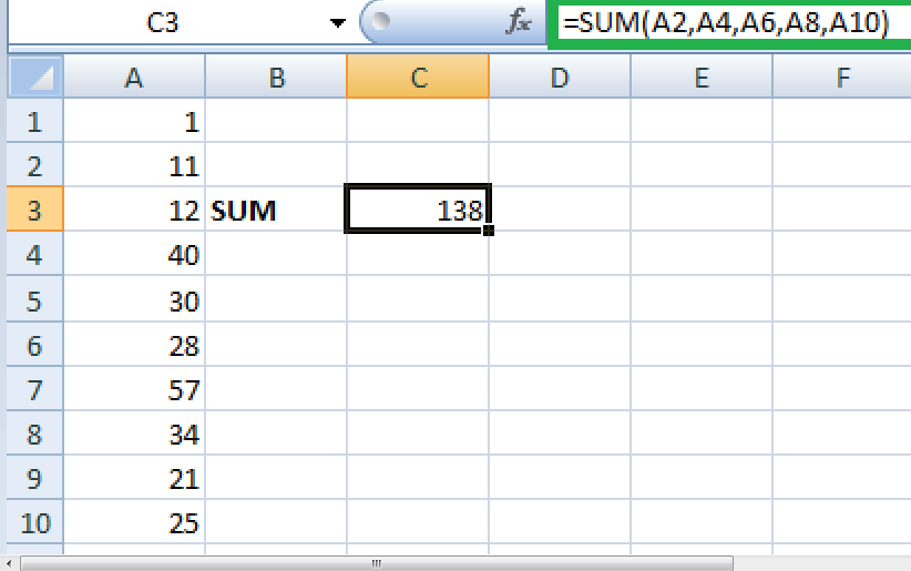
Here the result for the particular cell range is displayed as 138 which is the sum of A2, A4, A6, A8 and A10.
5. How to use AutoSum Function?
AutoSum in Excel is used to sum the column or row of numbers quickly. To use AutoSum Function following steps are followed.
Step 1: Enter the data in the spreadsheet
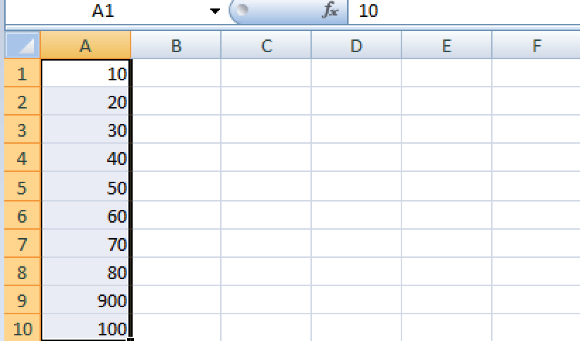
Step 2: Select the row or column of numbers to perform AutoSum function as shown in the above image.
Step 3: To execute Sum function in Excel, Choose AutoSum from Edit group in the Home Tab.

Step 4: By choosing AutoSum the result will be automatically displayed in the required column.
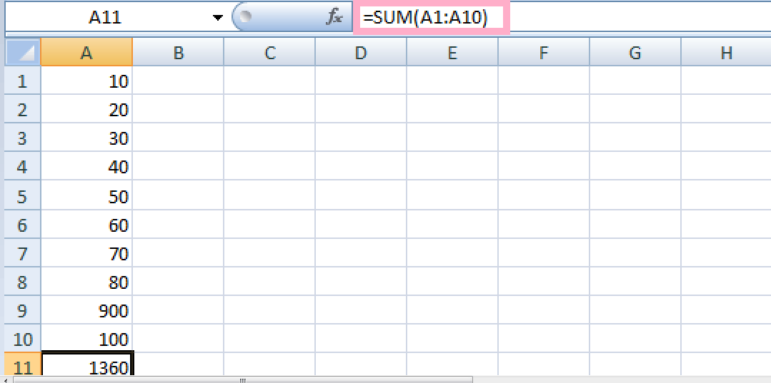
Step 5: One can choose AutoSum or by pressing (ALT+=). Similar method follows for adding the entire row.
Here is another example, how to sum the large sets of data in the Excel.
STEP 1: Enter the data in the Excel and select the data which to be added.
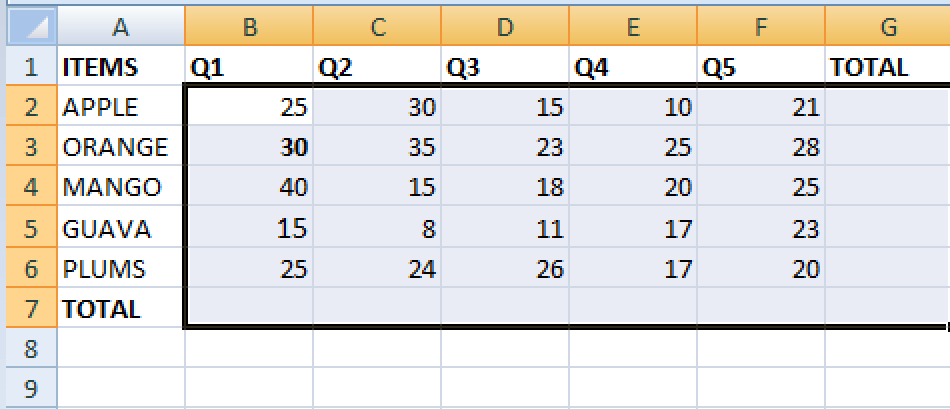
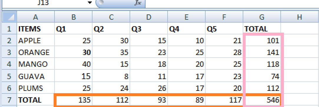
Step 2: Press (ALT+=). This function implements 8 SUM Functions. It totals the value of row wise and column wise.
6. How to Sum the range with Errors?
Sometimes, while adding a specified range, there is some error data in the cell. The sum and error function is used to sum the data except for the error data, and two functions, namely SUM and IFERROR, are used.
Step 1: Enter the data in the spreadsheet.
Step 2: Select the cell where the result wants to display and enter the formula as =SUM(IFERROR(A1:A7,0))
Step 3: After entering the formula press CTRL+SHIFT+ENTER.
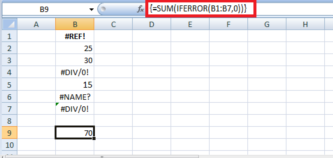
The result will be displayed as shown in the above worksheet which sums the value present in the text.
7. How to find Largest Numbers?
The data present in the cell is a combination of largest, smallest, even, odd, negative and positive. To sum the largest number, LARGE function is used. Here is an example to find the second largest number in the set of data present in the column.
Step 1: Enter the data in the specified column.

Step 2: Select the cell where you want to display the result and enter the formula as =LARGE (A1:A11, 2) where A1:A11 indicates the cell range and number 2 represents the second largest number.

Here the second largest number is displayed as 100 among various numeric values. To find the first largest number replaces the number two with one. Similarly, the user can find the required large number in the values.
8. How to Sum Largest Numbers?
In previous method how to find the largest method is discussed. Here in this method lets discuss how to the sum the largest number.
Step 1: Enter the data in the worksheet.

Step 2: Select the cell where the result want to display and type the formula as =SUM(LARGE(A1:A11,{1,2,3,4}))
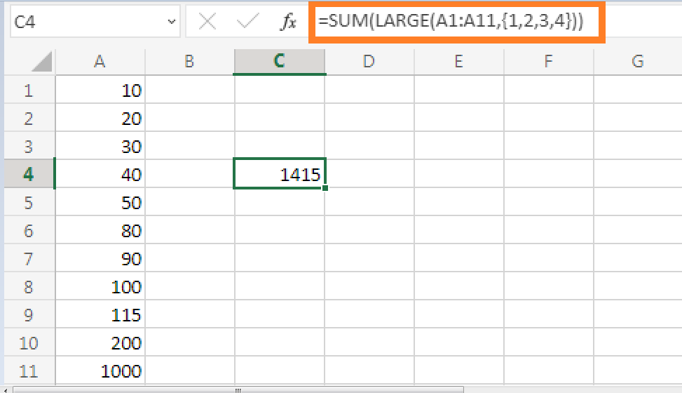
Here the result will be displayed as 1415, which is the sum of first four largest numbers as 1000+200+115+100=1415.
After inserting the formula in the cell, one can press Enter or by clicking CTRL+SHIFT+ENTER. The array function used in formula acts as a argument for the SUM function, which displays the result as 1415.
9. How to Sum Nth Row?
To sum the Nth row in a number, formula used is SUM, MOD and ROW. Sometimes the calculation needs to be sum nth row in the data. The steps to be followed to calculate the nth row of the data as follows.
Step 1: Enter the data in the spreadsheet
Step 2: Select the cell where the result want to display, enter the formula as {=SUM(A1:A11*(MOD(ROW(A1:A9),3)=0))}
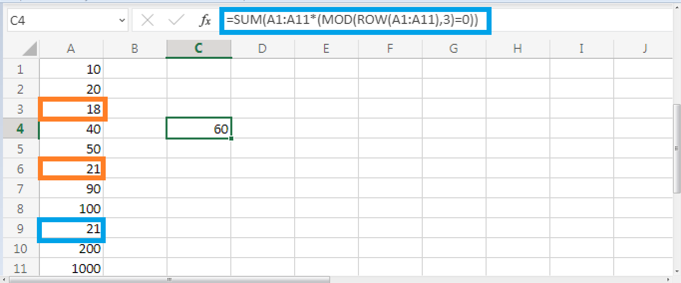
Here in the result are 60, which is the sum of every 3rd row such as 18+21+21=60. Similarly the user can add the every nth row by changing the number in the formula.
10. How to use Alternative method for SUM function?
The values are added either by using SUM function or using default functions present in the Excel. Here some of the alternative methods are mentioned, how to add the values using Excel functions.
Step 1: Enter the data in the spreadsheet.
Step 2: Click on the Formula tab, choose Math and Trig. A list of option will display in that choose the SUM value.
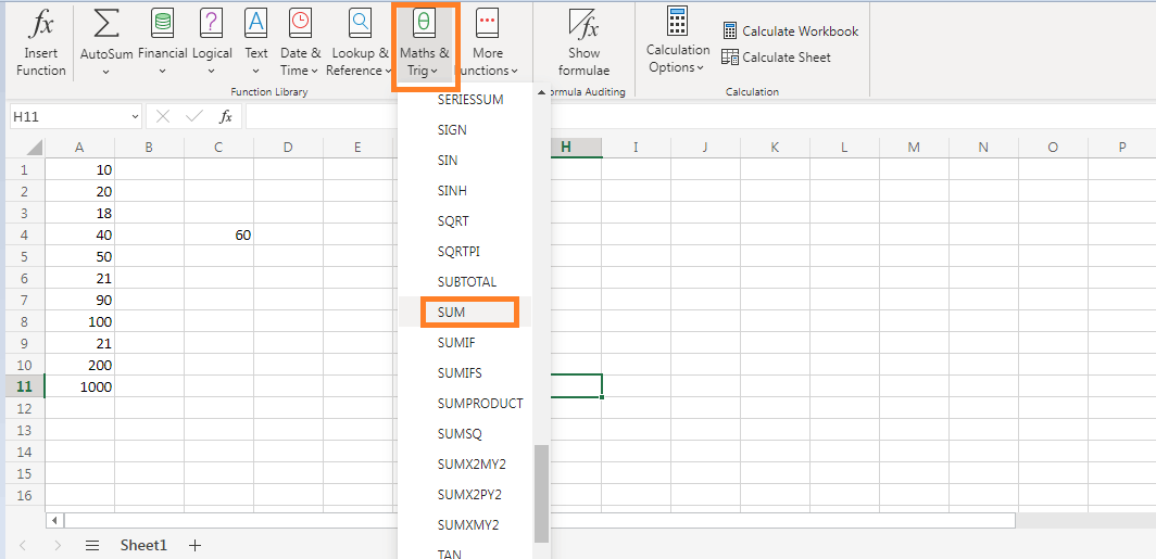
Step 3: After clicking the Sum, a cell is selected, in that enter the range which needs to be added.
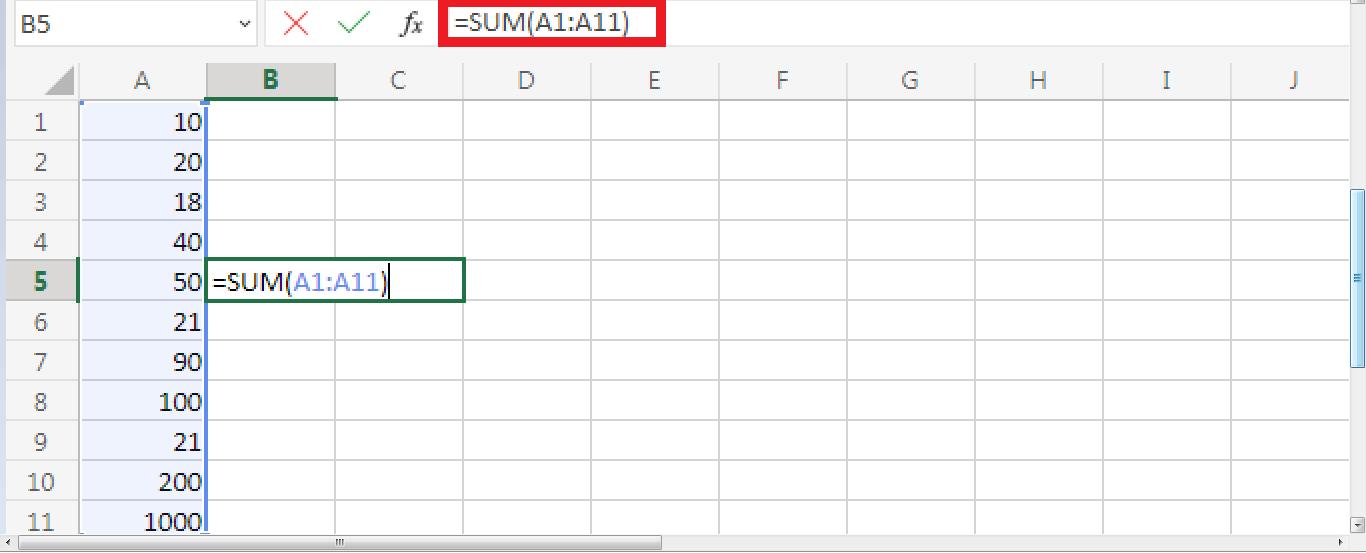
Here the range is entered as A1:A11 where the result will be displayed.
11. What is nesting functions in Excel?
Excel enables the function to use Nesting functions for performing multiple calculations. Nesting is the process where one function is nested inside the other function; hence, multiple and large calculations are performed in a single worksheet. The nested function is the argument of the main or the outermost function. Like mathematics, Excel calculates the innermost function first and the outermost function.
Some example of nested function is as follows,
=ROUND(SUM(A1:A6),3)
Here the range of cells A1:A6 is computed and the number 3 indicates the rounded to three decimal places.
Usage of Sum Functions
The usages of sum functions are,
1. The arguments in the functions contain arrays, numbers, cell references, constants, ranges and results of the various functions and formulas.
2. Numeric output is obtained where it denotes the sum of values present in the data.
3. The argument has its limit of about 255.
Limitations of Sum Function
Some of the limitations of sum function are,
1. Cell which contains the output must be in a number format.
2. The cell range supplied should match the dimension of the source.
Summary
From the tutorial, the various functions and formulas of the SUM function are explained briefly. Calculations regarding Sum may vary regarding data. Based on the requirement, the various formulas and functions are present default in Excel, like Sum the entire row, column, single row etc. The SUM functions return the Sum of values applied, which includes arrays, numbers, cell references, constants, ranges etc. By utilizing this function, the calculations are done quickly and effectively.