2D Arrays Application - Sparse Matrix

A matrix is a two-dimensional data item consisting of m rows and n columns, with a total of m x n values. A sparse matrix is one in which the majority of the entries have a 0 value.

Large sparse matrices are frequent in general and notably in applied machine learning, such as in data with counts, data encodings that map categories to counts, and even whole subfields of machine learning like natural language processing.

It is computationally costly to represent and deal with sparse matrices as if they were dense, therefore adopting representations and operations that properly address the matrix sparsity can result in significant performance gains.

It's named sparse because the density of non-zero items is minimal. When we save Sparse Matrix as a two-dimensional array, we waste a lot of space storing all those 0's explicitly. Furthermore, numerous operations on sparse matrices stored in a 2-dimension array, such as addition, subtraction, and multiplication, are performed on elements with zero values, resulting in significant time waste. Thus, directly storing the non-zero components is a superior technique, since it considerably decreases the amount of storage space and calculations necessary to conduct different operations.

Huge matrices are used in a broad variety of numerical problems in real-world applications such as engineering, science, computers, and economics. These matrices frequently contain a large number of zero elements, and matrices with a significant proportion of zero entries are known as sparse matrices.

Why use a sparse matrix rather than a simple matrix?

Storage: Because there are fewer non-zero items than zeros, less memory may be utilised to store solely those.
Computing time: It can be reduced by rationally constructing a data structure that only traverses non-zero items.

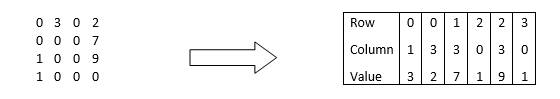
The usage of a 2D array to represent a sparse matrix wastes a lot of resources since the zeroes in the matrix are rarely used. As a result, we only save non-zero items instead of zeroes. This entails using triples to store non-zero items (Row, Column, value).

Example:

Finding the Sparse Matrix in C using arrays.

A two-dimensional array is used to create a sparse matrix with three rows designated as

Row: The index of the row in which the non-zero element is found.
Column: The index of the column in which the non-zero element is found.
Value: The value of the non-zero element at index – (row,column).

C code implementation

// C++ program for Sparse Matrix Representation
// using Array
#include<stdio.h>


int main()
{
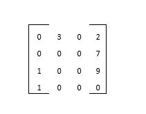
// Assume 4x4 sparse matrix
int s_matrix[4][5] =
{
{0 , 3 , 0 , 2 },
{0 , 0 , 0 , 7 },
{1 , 0 , 0 , 9 },
{1 , 0 , 0 , 0 }
};


int n = 0;
for (int i = 0; i < 4; i++)
for (int j = 0; j < 5; j++)
if (s_matrix[i][j] != 0)
n++;


// number of columns in compactMatrix (n) must be
// equal to number of non - zero elements in
// sparseMatrix
int c_matrix[3][n];


// Making of new matrix
int k = 0;
for (int i = 0; i < 4; i++)
for (int j = 0; j < 5; j++)
if (s_matrix[i][j] != 0)
{
c_matrix[0][k] = i;
c_matrix[1][k] = j;
c_matrix[2][k] = s_matrix[i][j];
k++;
}


for (int i=0; i<3; i++)
{
for (int j=0; j<n; j++)
printf("%d ", c_matrix[i][j]);


printf("\n");
}
return 0;
}

The following output should be generated by this programme:

Output

0 0 1 2 2 3 
1 3 3 0 3 0
3 2 7 1 9 1

Sparse Matrix Types

Sparse matrices can be classified according to their sparsity. Sparse matrices may be defined using these features.

Regular sparse matrices
Irregular sparse matrices / Non - regular sparse matrices

Sparse matrices with regular sparsity

A regular sparse matrix is a square matrix with a well-defined sparsity pattern, which means that non-zero items appear in a predictable sequence. The following are the numerous types of regular sparse matrices:

Sparse matrices with lower triangular regularity
Sparse matrices with upper triangular regularity
Sparse matrices with three diagonals

Sparse matrices with lower triangular regularity.

Lower regular sparse matrices have all members above the main diagonal with zero values. The matrix below is a lower triangular regular sparse matrix.

Lower triangular regular sparse matrices are stored.

The non-zero entries of a lower triangular regular sparse matrix are stored in a 1-dimensional array row by row.

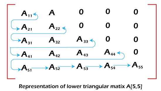
As an example: The one-dimensional array X stores the 5 by 5 lower triangular regular sparse matrix depicted in the preceding figure:

X = {A₁₁, A₂₁, A₂₂, A₃₁, A₃₂, A₃₃, A₄₁, A₄₂, A₄₃, A₄₄, A₅₁, A₅₂, A₅₃, A₅₄, A₅₅ }

To determine the total number of non-zero items, we must first determine the number of non-zero elements in each row, then add them together. Since the number of non-zero components in an ith row is:

1 + 2 + ………………… + i + ………………….. + (n-1) + n = n (n+1)/2

Sparse matrices with upper triangular regularity.

All of the entries below the main diagonal are zero in the upper triangular regular sparse matrix. The Upper triangular regular sparse matrix comes next.

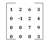
Upper triangular regular sparse matrices storage.

The non-zero elements of an upper triangular regular sparse matrix are stored in a 1-dimensional array column by column in an upper triangular regular sparse matrix.

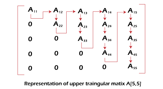
The 5 by 5 lower triangular regular sparse matrix, for example, is stored in one-dimensional array X, as illustrated in the preceding figure:

X = {A₁₁, A₂₁, A₂₂, A₃₁, A₃₂, A₃₃, A₄₁, A₄₂, A₄₃, A₄₄, A₅₁, A₅₂, A₅₃, A₅₄, A₅₅}

To compute the total number of non-zero items, we must first determine the number of non-zero elements in each row, then add them together. Since the number of non-zero items in the ith row is equal to the total number of non-zero elements in the lower triangular regular sparse matrix of n rows, the total number of non-zero elements in the lower triangular regular sparse matrix

1 + 2 + ………………… + i + ………………….. + (n-1) + n = n (n+1)/2

Sparse matrices with three diagonals.

All non-zero entries of the tridiagonal regular sparse matrix reside on one of the three diagonals, the main diagonal above and below.

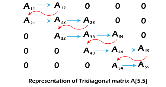
Storing regular tri-diagonal sparse matrices.

All non-zero entries in a tri-diagonal regular sparse matrix are stored in a 1-dimensional array row by row.

The 5 by 5 tri-diagonal regular sparse matrix, for example, is stored in one-dimensional array D, as illustrated in the following figure:

D = { A₁₁, A₁₂, A₂₁, A₂₂, A₂₃, A₃₂, A₃₃, A₃₄, A₄₃, A₄₄, A₄₅, A₅₄, A₅₅}

We need to know the number of non-zero items on the diagonal, above the diagonal, and below the diagonal in order to determine the total number of non-zero elements. A square matrix has n items along the diagonal and n elements above the diagonal (n-1). In an n-square matrix, the total number of non-zero components is:

n + (n-1) + (n-1)

the diagonal Above the diagonal Below the diagonals

As a result, given an n-squre matrix, the total number of entries is 3n-2.

Now, if we take n=7, the total number of pieces is 3 * 7 - 2 = 19.

Sparse matrices with irregularities

The irregular sparse matrices are those with an irregular or unstructured pattern of non-zero element occurrences. The matrices below are irregular sparse matrices.

There are various typical storage techniques for sparse matrices shown in the picture above. The majority of these systems store all of the matrix's non-zero members in a 1-dimensional array.

Irregular sparse matrices storage schemes:

The non-zero components of the matrix are stored in a 1-dimensional array, and the position of non-zero elements in the sparse matrix is specified using various auxiliary arrays. The following are the most typical storage strategies for irregular sparse matrices among the many options:

Index Method of Storage
Compressed Row Format Storage

Using the Index Method to store an irregular sparse matrix

We can store irregular sparse matrices A using the index approach by creating three 1-Dimensional arrays AN, AI, and AJ, each with elements equal to the total number of non-zero components.

The non-zero items are stored in the array AN in a row-by-row fashion.
A[I, J] in matrix A holds the appropriate row number of non-zero entries AI.
A[I, J] in matrix A includes the appropriate column number of non-zero items AJ.

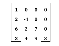
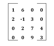
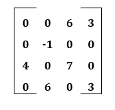
Consider the following sparse matrix A, which is 4 by 4:

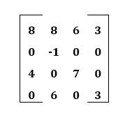
Only 9 of the 16 entries in this Sparse Matrix are non-zero. The following are non-zero elements:

X [0, 0] = 8
X [0, 1] = 8
X [0, 2] = 6
X [0, 3] = 3
X [1, 1] = -1
X [2, 0] = 4
X [2, 2] = 7
X [3, 1] = 6
X [3, 3] = 3

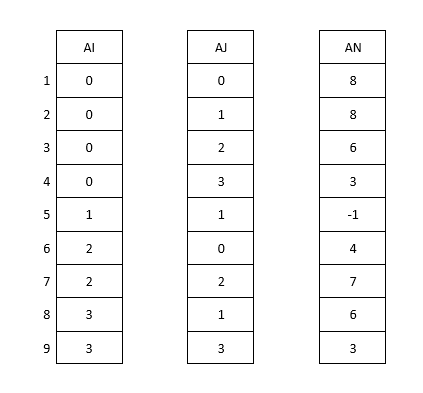
Three 1 - D arrays are represented in this diagram. AI, AJ, AN

Use the storage by index technique to save it. As indicated in the picture, we create three-dimensional arrays AN, SI, and AJ, each with 9 elements (i.e., the total number of non-zero elements).

The non-zero items are stored consecutively in the array AN. Each non-zero element's matching row and column numbers are kept in arrays AI and AJ, respectively.

Using the compressed row storage format to store irregular sparse matrices

Compressing row storage is another space-efficient and extensively used approach for expressing irregular sparse matrices. Three 1-Dimensional arrays, AN, AI, and AJ, are used in this method. The non-zero element values are extracted row-wise from the matrix and stored in the one-dimensional array AN. The original column locations of the matching items in AN are stored in the next 1-dimensional array AJ, which has the same length as AN. The position of the first entry of non-zero elements in an array is stored in a 1-dimensional array AI with a length equal to many rows.

For instance:

AI [2] = 4 indicates that the first non-zero elements in row 2 are stored in AN[4], which is 2.
We build three 1-dimensional arrays, AN, AI, and AJ, as indicated in the following image, to store it using compressing row storage format:

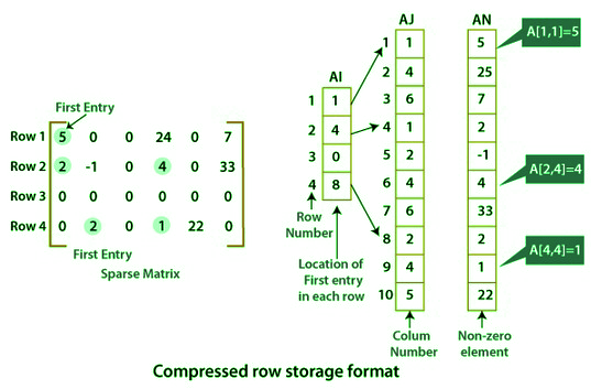
The array AN has ten non-zero entries that are stored in a row-wise order. In the 1-dimensional array AJ, the relevant column numbers are recorded. The entries in the 1-dimensional array AI point to the first non-zero member of each row in arrays AJ and AN.

Data Structures Tutorial

Misc Topic: