Types of Data Structures

Almost every programme or software system that has been built makes use of data structures. Furthermore, data structures are basics of computer science and software engineering. When it comes to Software Engineering interview questions, this is a critical issue. As a result, as developers, we must be well-versed in data structures.

We've spoken about data types and data structure classifications so far. Our journey through the many aspects of data structures continues with an examination of the various forms of data structures.

Arrays

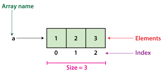
Arrays are groups of data elements of the same kind that are stored in adjacent memory regions. Each data piece is referred to as a "element." Arrays are the most fundamental and basic data structure. Before going on to other structures like as queues or stacks, aspiring Data Scientists should grasp array creation.

An array is a fixed-size structure. It can be an array of integers, a floating-point number array, a text array, or even a collection of arrays (such as 2-dimensional arrays). Because arrays are indexed, they may be accessed at any time.

Operations on arrays

• Traverse: Print the elements as you go through them.
• Search: Search the array for a certain element. You may look for an element by its value or index.
• Update: Updates the value of an existing element at a specified index.

Because arrays are fixed in size, adding and removing elements to and from them cannot be done immediately. To add an element to an array, you must first build a new array with a larger size (current size + 1), copy the existing items, and then add the new element. The same is true for deleting an array and replacing it with a smaller one.

Graphs

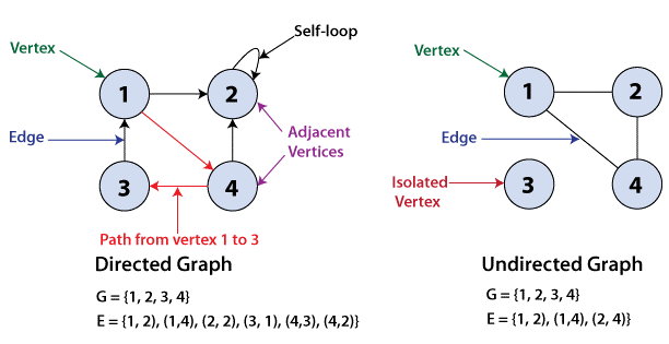
Graphs are illustrative nonlinear representations of element sets. Graphs are made up of finite node sets, also known as vertices that are connected by connections, also known as edges. Trees, as indicated below, are a type of graph with no rules dictating how the nodes join.

The number of vertices in a graph determines its order. The number of edges in a graph determines its size.

If two nodes are connected by the same edge, they are said to be neighbouring.

Directed Graphs

A graph G is said to be a directed graph if all of its edges have a direction specifying which vertex is at the beginning and which vertex is at the conclusion.

(u, v) is said to be incident from or exits vertex u and incident to or enters vertex v.

Self-loops are edges that connect a vertex to itself.

Undirected Graphs

If all of the edges of a graph G have no direction, the graph is said to be undirected. It can go in both directions between the two vertices.

A vertex is considered to be isolated if it is not linked to any other node in the graph.

Hash Tables

Hash tables, also known as hash maps, can be utilised as a linear or nonlinear data structure, albeit the former is preferred. Arrays are typically used to construct this structure. Hash tables are used to map keys to values. For example, every book in a library is allocated a unique number, which makes it easier to seek up information about the book, such as who has checked it out, its current availability, and so on. The library's books are hashed to a unique number.

Furthermore, if we know the key associated with the value, it provides efficient lookup. As a result, regardless of the amount of the data, it is highly efficient at inputting and searching.

When putting data in a table, Direct Addressing employs a one-to-one mapping between values and keys. When there are a high number of key-value pairs, however, this strategy has a difficulty. Given the memory available on a standard computer, the table will be enormous with so many records and may be difficult or even impossible to store. Hash tables are used to prevent this problem.

Using the Hash Function

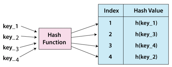
To circumvent the aforementioned difficulty with direct addressing, a special function called the hash function (h) is utilised.

A value with key k is stored in the slot k in direct accessing. We compute the index of the table (slot) to which each item belongs using the hash function. The hash value for a particular key is the value calculated using the hash function, and it shows the index of the table to which the data is mapped.

h(k) = k % m

• h: stands for hash function.
• k: The key for which the hash value is to be calculated.
• m: hash table's size in millimetres (number of slots available). A prime number that isn't quite a power of two is an excellent candidate for m.

When the hash function yields the same index for several keys, a collision might occur. Collisions can be avoided by using a proper hash function h and strategies like chaining and open addressing.

Linked List

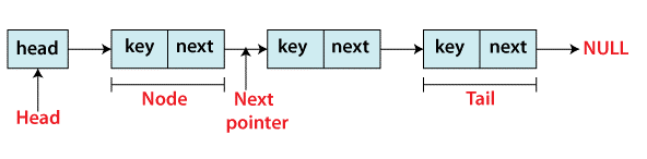
Linked lists keep item collections in a sequential sequence. Each linked list element contains a data item as well as a link, or reference, to the next item on the same list.

As a result, you must access data in a specific order; random access is not feasible. Linked lists are a simple and versatile way to express dynamic sets.

Consider the following words in the context of linked lists.

• Nodes are the elements of a linked list.
• Each node has a key and a reference to the next node, which is its successor.
• The head property refers to the first item in the linked list.
• The tail is the final member of the linked list.

The many forms of linked lists accessible are shown below.

• Singly Linked List - Only forward traversal of items is possible with a single linked list.
• Doubly Linked List - Traversing items in both forward and backward directions is possible using a doubly linked list. Prev is an additional pointer on nodes that points to the previous node.
• Circular Linked List - Circular linked lists are linked lists in which the head's previous pointer links to the tail and the tail's next pointer points to the head.

Operations on linked lists

• Search: Using a basic linear search, find the first entry in the supplied linked list with the key k and return a reference to that element.
• Insert: To the connected list, add a key. Insertion can be done in one of three ways: at the start of the list, at the end of the list, or in the middle of the list.
• Delete: Removes a provided linked list entry x. A node cannot be deleted in a single step. A deletion can be performed in one of three ways: from the start of the list, from the end of the list, or from the middle of the list.

Stack

A stack is a Last In First Out (LIFO) (Last In First Out – the element put last may be retrieved first) structure found in many programming languages. Because it resembles a real-world stack – a stack of plates — this form is called "stack."

Operations on the stack

The two fundamental operations that may be done on a stack are listed below.

• Push: Push an element to the very top of the stack.
• Pop: Remove the topmost element and replace it with a new one.

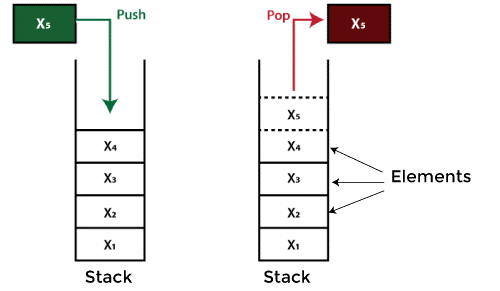
In order to verify the state of a stack, the following extra functions are available.

• Peek: Returns the stack's top member without destroying it.
• isEmpty: Determines whether the stack is empty.
• isFull: Determines whether the stack is full.

Queue

Queues, like stacks, store item collections sequentially, but the operation order must be "first in, first out." Queues are essentially linear lists.

Because it resembles a real-world queue – individuals waiting in a line — this structure is called "queue."

Operations involving queues

The two fundamental operations that may be done on a queue are listed below.

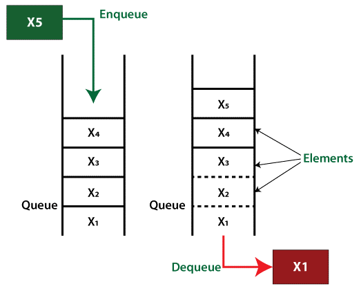
• Enqueue: Add a new element to the queue's end.
• Dequeue: Remove the element from the queue's beginning.

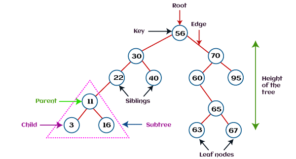
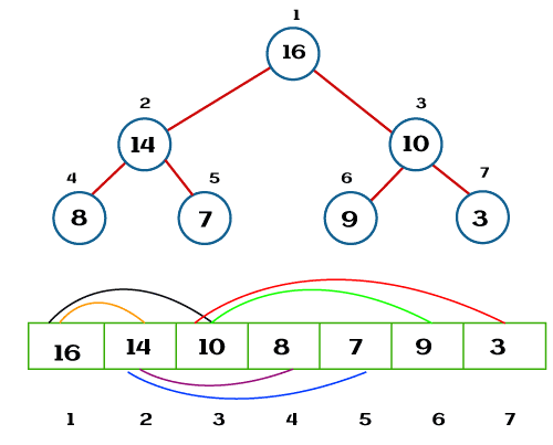
Tree

Trees are abstract hierarchies that hold item collections. They are node-based multilevel data structures. The lowest nodes are referred to as "leaf nodes," while the highest node is referred to as the "root node." Each node has references to neighbouring nodes. This structure differs from that of a linked list, in which elements are connected in a linear order.

Various sorts of trees have been produced throughout the years to suit certain uses and to fulfil specific limits. Binary search tree, B tree, treap, red-black tree, splay tree, AVL tree, and n-ary tree are some examples.

Binary Search Tree

A binary search tree (BST) is a binary tree in which data is structured in a hierarchical structure, as the name implies. The values in this data structure are stored in sorted order.

In a binary search tree, each node has the following qualities.

• Key: The value stored in the node's key.
• left: The pointer is pointing at the youngster on the left.
• right: The pointer to the kid on the right.
• p: The parent node's pointer.

A binary search tree has a distinguishing feature that sets it apart from other trees. The binary-search-tree property is the name for this property.

In a binary search tree, let x be a node.

• When y is a node in x's left subtree, then y.key is  ≤ x.key.
• When y is a node in x's right subtree, y.key ≥ x.key.

Trie

Tries, which are not to be confused with Trees, are data structures that hold strings as data elements and are organised in a visual graph. Attempts are also known as keyword trees or prefix trees. You can see the trie data structure in action whenever you use a search engine and get auto recommendations.

Heaps

A heap is a type of binary tree in which the parent nodes' values are compared to those of their offspring and the nodes are sorted accordingly.

There are two sorts of heaps.

• Min Heap - The parent's key is less than or equal to that of its children in the Min Heap. The min-heap property is what it's called. The heap's minimum value will be stored in the root.
• Max Heap - the parent's key is larger than or equal to the children's. The max-heap property is what it's called. The heap's maximum value will be stored in the root.