Tim Sort
Tim Sort is a mixture stable arranging calculation that exploits normal examples in information, and uses a mix of an improved Merge sort and Binary Insertion sort alongside an interior rationale to upgrade the control of enormous scope true information.
Tim Sort was first carried out in 2002 by Tim Peters for use in Python.
Operation Status:
Tim sort utilizes Binary insertion sort and improved blend sort by utilizing running in a mix. Paired inclusion sort is the best strategy to sort when information is or to some degree arranged or the length of run is more modest than MIN_RUN and blend sort is best when the information is enormous.
Tim Sort is intricate, even by algorithmic guidelines.
The activity is best separated into parts:
Run(Division operation):
An info exhibit is partitioned into various sub-clusters, count of components inside a sub-cluster is characterized as a RUN, the base worth of such runs is a MIN_RUN which is a force of 2 not a bigger number of than 32 (or 64).
These sub-clusters are normally somewhat requested (rigorously rising or stricly descending).
When the exhibit is disintegrated into a few runs, the runs of climbing request stay unaltered, and the runs of stringently plummeting request are switched.
At last, a few runs of rising request are gotten.
Example:
Think about a variety of objectives:
1 5 9 8 6 4 5 6 7
We can see that [1, 5, 9] adjusts to climbing request, [8, 6, 4] adjusts to severe plummeting request, [4, 5, 6, 7] adjusts to rising request.
Flip the numbers in descending order:
1 5 9 6 8 4 5 6 7
Merging:
We should accept that the new exhibit is:
.... 6 7 8 9 10 1 2 3 4 ....
Assuming that we combine two runs utilizing Mergesort alone
run1: [6, 7, 8, 9, 10]
run2: [1, 2, 3, 4, 5]
Mergesort thinks about the primary component of the two runs
1 < 6, get 1
2 < 6, get 2
3 < 6, get 3
4 < 6, get 4
5 < 6, get 5
We found that navigating the whole run straightforwardly would ultimately consume more number of consolidation activities assuming the run was longer.
Since each run is in climbing request, there's compelling reason need to look at them individually and the idea of Galloping becomes convenient.
Galloping:
For instance, to consolidate the accompanying two runs:
run1: [101, 102, 103, ... 200]
run2: [1, 2, 3, ..., 100]
Rather than contrasting the components individually, we analyze them by expanding powers of 2^n where n >= 0.
run1[0] > run2[0]
run1[0] > run2[1]
run1[0] > run2[3]
run1[0] > run2[7]
run1[0] > run2[15]
...
run1[0] > run2[2^n - 1]
run1[0] <= run2[2^(n+1) - 1]
We come by an outcome run2 [2 ^ n - 1] < run1[0] <= run2 [2 ^ (n + 1) - 1],
Since run2 is arranged, we utilize Binary Search to find run1[0] in run2 effectively by characterizing left = run2[2^n - 1], right = run[2^(n+1) - 1].
Thus the times we combine two runs is diminished from O(N) to O(logN).
Note:
Why not skip Galloping and simply do Binary Search?
How about we give a model:
run1: [1, 3, 5, 7, 9 ... 2n+1]
run2: [0, 2, 4, 6, 8 ... 2n]
Along these lines, run1[0] is just bigger than run2[0]. Each time we do Binary Search, we can get various outcomes, in addition to n seasons of Binary Search, so the time intricacy changes from O(N) to O(NlogN).
Stack:
At the point when the first cluster turns into a bunch of different climbing runs, we really want to consolidate two runs, yet in the event that we combine a long run with a more limited run, it will require a more extended investment to look at a comparitively more limited run.
So Timsort keeps a stack with every one of the run lengths on the stack, while fulfilling that the length of run on the back stack is longer than the amount of the length of run on the initial two stacks, so the length of run generally diminishes.
Stack : [... runA, runB, runC]
runA > runB + runC
runB > runC
This keeps away from run converges with an excess of distinction long.
For the individuals who favor shots:
Lay out a minrun size that is a force of 2 (normally 32, never more than 64 or your Binary Insertion Sort will lose productivity)
Find a disagreement the first minrun of information.
On the off chance that the run isn't basically minrun long, use Insertion Sort to snatch resulting or earlier things and addition them into the run until it is the right least size.
Rehash until the whole cluster is partitioned into arranged subsections.
Utilize the last 50% of Merge Sort to join the arranged exhibits.
Complexity Analysis:
By plan TimSort is appropriate for to some extent arranged information with the best case being completely arranged information. It falls into the versatile sort family. Taking the quantity of runs ρ as a (characteristic) boundary for a refined investigation we got:
- TimSort runs in O(N + Nlogρ) time.
- Worst case time complexity: O(NlogN)
- Average time complexity: O(NlogN)
- Best case time complexity: O(N)
- Space complexity: O(N)
Applications of Tim sort:
1.Tim Sort is strong. It is quick and stable, however maybe in particular it exploits certifiable examples and uses them to fabricate an eventual outcome.
2.Tim Sort is utilized as the default arranging calculation in Java's Arrays.sort() technique, Python's arranged() and sort() strategies, the Android Platform, and in GNU Octave.
3.At the point when the info is arranged, Tim Sort runs in direct time, implying that it is a versatile arranging calculation.
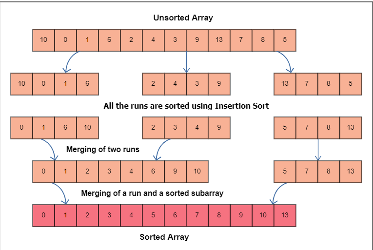
Visual Representation:
//program
minrun = 32
def InsSort(arr1,start1,end1):
    for 1 in range(start1+1,end1+1):
        elem1 = arr1[i]
        j = i-1
        while j>=start1 and elem1<arr1[j]:
            arr1[j+1] = arr1[j]
            j - = 1
        arr1[j+1] = elem1
    return arr1
def merge(arr1,start1,mid1,end1):
    in the event that mid1==end1:
        return arr1
    first1 = arr1[start1:mid1+1]
    last1 = arr1[mid1+1:end1+1]
    leng1 = mid1-start1+1
    leng2 = end1-mid1
    index1 = 0
    index2 = 0
    ind = begin


    while index1<leng1 and index2<leng2:
        if first1[index1]<last1[index2]:
            arr1[index] = first1[index1]
            indeex1 += 1
        else:
            arr1[index] = last1[index2]
            index2 += 1
        index += 1


    while index1<leng1:
        arr1[index] = first1[index1]
        index1 += 1
        index += 1


    while index2<leng2:
        arr1[index] = last1[index2]
        index2 += 1
        index += 1


    return arr1


def TimSort(arr1):
    n = leng(arr1)


    for start in range(0,n,minrun):
        end1 = min(start1+minrun-1,n-1)
        arr1 = InsSort(arr1,start1,end1)


    curr_size = minrun
    while curr_size<n:
        for start in range(0,n,curr_size*2):
            mid = min(n-1,start+curr_size-1)
            end = min(n-1,mid+curr_size)
            arr = merge(arr,start,mid,end)
        curr_size *= 2
    return arr
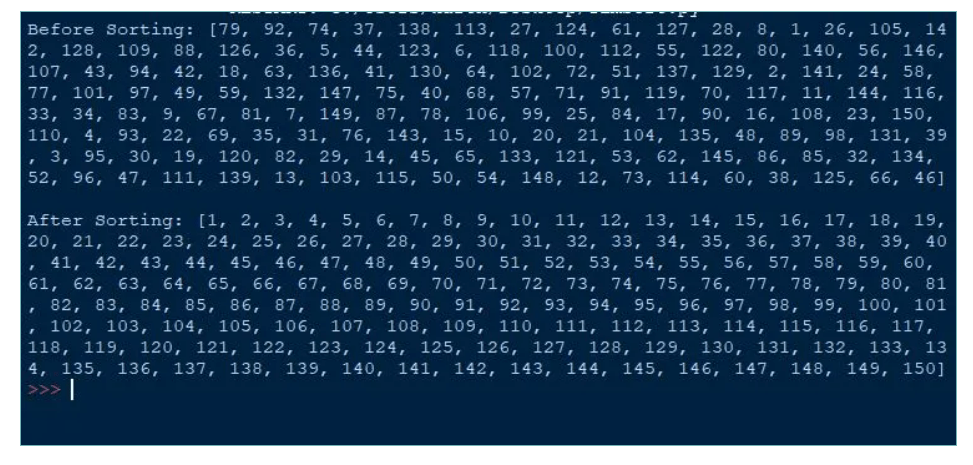
Output: