Bubble Sort vs Quick Sort

In this article, we are going to compare two sorting techniques, Bubble sort and Quick Sort. In starting, we will first discuss the idea of sorting an array using bubble sort and quick sort both, and later on, we will discuss their differences.

Let’s start the discussion with the Bubble sort:

Q. Discuss the idea of bubble sort through an example:

Bubble sort - The bubble sort is a ‘subtract and conquer’ based sorting technique. In which it continuously compares all the elements and places all the elements in their right order. It is called bubble sort because it only compares two adjacent elements referred to as the bubble at any instant.

On each complete iteration of the internal for loop, the largest element is placed at the last index of the unsorted part of the array.

The pseudo-code of the Bubble Sort Function:

1. Bubble Sort (A, N)
2.	For I = 1 to N - 1
3.		For J = 0 to N - I – 1
4.			If A[J] > A[J + 1]
5.				Swap (A[J], A[J + 1])
// Where N represents the number of elements present in the array A.

// Where N represents the number of elements present in the array A.

In the above pseudo-code, we have nested for-loops. The internal for-loop starts and ends at 0 and N – I – 1, respectively, and the external for-loop starts and ends at 1 and N – 1, respectively. The if-block checks if the element at the right is smaller than the element at the left and swaps them if the condition is satisfied.

Now, let us sort a sample array to get a complete overview of the bubble sort.

Consider an array A[] = {17, 12, 16, 4, 3} with five elements passed to the bubble sort function. The steps involved in sorting the given array using bubble sort are listed below:

1. First iteration of External For-Loop – I = 1. The internal for loop starts from 0 and ends at 5 – 1 – 1 = 3.

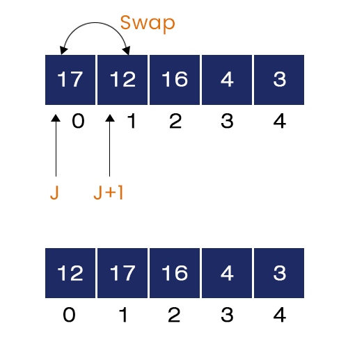
• First Iteration of Internal For-Loop, J = 0.
  Here, A[J] = 17 and A[J + 1] = 12 and 17 > 12. Hence, the if-condition is true. We swap them, and the 17 and 12 are now placed in ascending order.

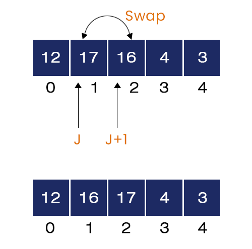
• Second Iteration of Internal For-Loop, J = 1.
  Here, A[J] = 17 and A[J + 1] = 16 and 17 > 16. Hence, the if-condition is true. We swap them, and the 17 and 16 are now placed in ascending order.

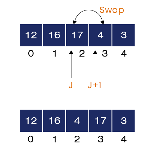
• Third Iteration of Internal For-Loop, J = 2.
  Here, A[J] = 17 and A[J + 1] = 4 and 17 > 4. Hence, the if-condition is true. We swap them, and the 17 and 4 are now placed in ascending order.

• Fourth Iteration of Internal For-Loop, J = 3.
  Here, A[J] = 17 and A[J + 1] = 3 and 17 > 3. Hence, the if-condition is true. We swap them, and the 17 and 3 are now placed in ascending order.

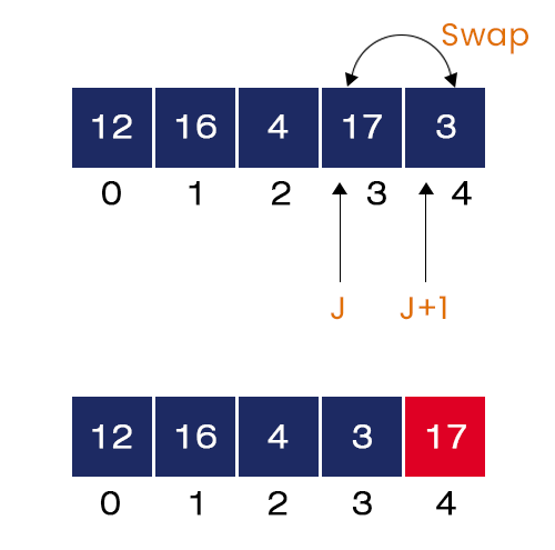
We can see that the largest element = 17, has finally taken his place. Now, we have the unsorted array of size N - 1 = 4. We repeat the same process for the remaining elements, same as above.

2. Second Iteration of External For-Loop, I = 1

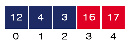
In this iteration, the second largest value = 16 will be placed at the index = 3, as shown in the figure.

3. Third Iteration of External For-Loop, I = 2

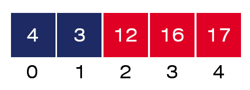
In this iteration, the third largest value = 12 will be placed at the index = 3, as shown in the figure.

4. Fourth Iteration of External For-Loop, I = 3

In this iteration, the fourth largest value = 4 will be placed at the index = 1. Also, the smallest value takes its position at index = 0, as shown in the figure below:

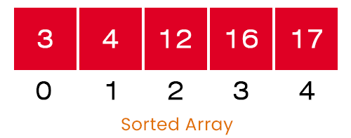
At the end of all the iterations of the external for loop, we have a sorted array as the program’s output.

Now, let us move to the idea of Quick Sort:

Q. Discuss the idea of Quick Sort with an example.

Quick Sort – The quick sort algorithm uses the ‘divide and conquer’ technique to sort several elements. The quick sort selects a random pivot element and places all the elements smaller than the pivot on its left side and all the elements greater than the pivot on its right side. By doing so, the pivot element reaches its correct position in the array. Now, the problem is divided into two subarrays which are the left subarray and right subarray. The quick sort repeats the same process on the left and right subarrays recursively until the array gets sorted.

The idea of selecting a good pivot element – The performance of the quick sort totally depends on the nature of the pivot element. A good pivot element enhances the performance of the quick sort. The way to select the pivot element is to choose the first, middle or last element as the pivot. But there is no best way to find a good pivot element. The better the randomness of elements, the better the chance to get a good pivot element.

Now, let us see the pseudo-code of the Quick Sort. The quick sort algorithm consists of two function blocks: the partition function and the quick sort function.

The pseudo-code of the Quick Sort function:

1. Quick Sort (A, L, R)
2.	If (L < R)
3.		Q = partition (A, L, R)
4.		Quick Sort (A, L, Q - 1)
5.		Quick Sort (A, Q + 1, r)


// L -> The left index of the array
// R-> The right index of the array

In the above pseudo-code, the quick function first calls the partition function and stores the index return by the partition function in Q and calls itself two times: Quick Sort (A, L, Q - 1) and Quick Sort (A, Q + 1, R).

The pseudo-code of the partition function:

1. Partition (A, L, R)
2.	Pivot = A[R]
3.	I = L -1
4.	for J = 0 to R - 1
5.		If (A[J] <= Pivot)
6.			I = I + 1
7.			Swap (A[I] and A[J])
8.	Swap (A[I + 1] and A[R])
9.	Return i + 1 // Index of the pivot element

The partition function compares the pivot element with all the values, makes necessary swapping, places the pivot element at its correct position in the array, and returns its index to the quick sort function.

Now, let us understand the idea of the quick sort function:

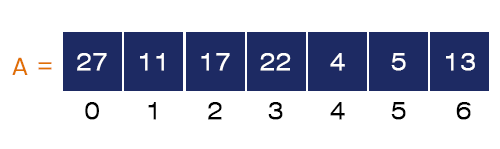
Consider an unsorted array A[] = {27, 11, 17, 22, 4, 5, 13} with seven elements in it. The steps involved in sorting the given array using the quick sort are listed below:

1. Quick Sort (A, 0, 6) is called
   The quick sort function first calls the Partition function (A, 0, 6). Let us first see the steps of the partition function.
   
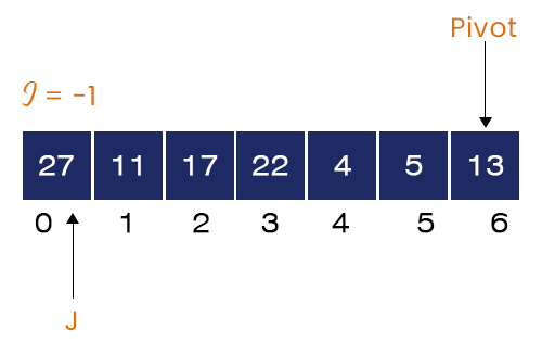
   Partition (A, 0, 6) is called – Here, the partition function selects the last element as the pivot element, Pivot = A[R] = A[6] = 13 and sets the value of I = L – 1 = 0 -1 = -1. Now, the for-loops starts from J = 0 to 6 - 1 = 5.

• When J = 0
  Here, A[J] = 27 which is greater than the Pivot = 13. So, the if-condition fails, no changes occur in this iteration.

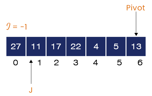
• When J = 1
  Here, A[J] = 11 which is less than the pivot = 13. So, the if-condition is true. Updating the value of I = -1 + 1 = 0 and swapping A[I] = 27 and A[J] = 11.

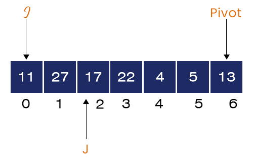
• When J = 2
  Here, A[J] = 17 which is greater than the Pivot = 13. So, the if-condition fails, no changes occur in this iteration.

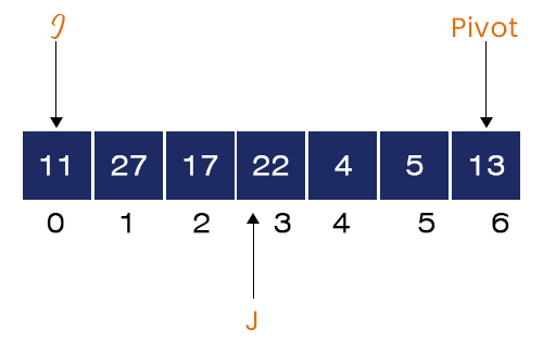
• When J = 3
  Here, A[J] = 22 which is greater than the Pivot = 13. So, the if-condition fails, no changes occur in this iteration too.

• When J = 4
  Here, A[J] = 4, which is less than the pivot = 13. So, the if-condition is true. Updating the value of I = 0 + 1 = 1 and swapping A[I] = 27 and A[J] = 4.

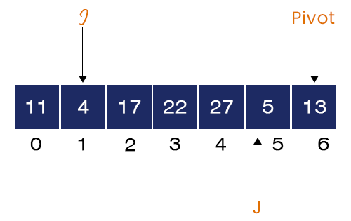
• When J = 5
  Here, A[J] = 5
  Here, A[J] = 5 which is less than the pivot = 13. So, the if-condition is true. Updating the value of I = 1 + 1 = 2 and swapping A[I] = 17 and A[J] = 5.

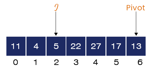
Now, swapping A[I + 1] = 22 and A[R] = 13.

As we can see, the elements on the left side of the pivot are smaller, and the elements on the right side are larger. Hence, the pivot is placed at its correct position in the array.

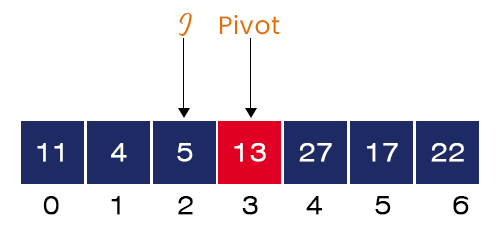
The partition function returns the index of the pivot element which is I = 2 + 1 = 3. And the control is again transferred to the quick sort function.

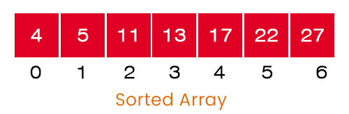
2. Here, the quick sort function calls itself on the left and right subarrays. The left and right subarrays are treated as the same problem separately. The quick sort algorithm repeats the same steps on them.

After complete execution of all the function calls, we get the desired sorted array as shown below:

Let us discuss the differences between sorting an array using Bubble Sort and Quick Sort. The main differences between these two sorting algorithms are listed below in the table:

	Bubble Sort	Quick Sort
Definition	The idea of bubble sort is to compare the adjacent elements one by one and maintain the required order between them.	The idea of quick sort is to select a random pivot element, place smaller elements left to the pivot and larger elements right to the pivot, and repeat the same process for the left and right parts recursively.
Approach	Subtract and conquer	Divide and conquer
Time Complexities	Best case: T(n) = O(n), Average case: T(n) = O(n ^ 2) Worst case: T(n) = O(n ^ 2)	Best case: T(n) = O(n logn), Average case: T(n) = O(n logn) Worst case: T(n) = O(n ^ 2)
Best-case and worst-case comparison	When we pass a sorted array, its flag version detects the sorted nature of the element in the single run and achieves the linear time complexity, O(n).	When we pass a sorted array, it starts behaving like the subtract and conquer sorting techniques, and its time complexity becomes O(n^2). This is because it always selects the minimum and maximum element as the pivot, and the problem size becomes equal to n-1 after the first call of the partition function.
Recurrence Relation	T(n) = T(n - 1) + n	T(n) = 2T(n / 2) + n
Stability	Stable – The order of similar elements remains unchanged.	Unstable – The order of similar elements may change.
Complexity	The complexity is very low in comparison to quick sort.	It is the most complex sorting algorithm among all six fundamental sorting algorithms.
Memory	Less space is required.	More space is required to manage the function calls.
Space Type	Internal	Internal
Method	Exchanging	Partition
Speed	Slower	Faster