Big O Notations

What is Big O Notation, and why is it important?

"Big O notation is a mathematical notation that depicts a function's limiting behaviour when the input tends towards a certain value or infinity." It belongs to the Bachmann–Landau notation or asymptotic notation family, which was established by Paul Bachmann, Edmund Landau, and others.

Big O notation, in a nutshell, expresses the complexity of your code in algebraic terms.

To understand Big O notation, consider the following example: O(n²), which is generally called "Big O squared." The letter "n" denotes the input size, and the function "g(n) = n²" within the "O()" indicates how difficult the algorithm is in relation to the input size.

The selection sort algorithm is an example of an algorithm with an O(n²) complexity. Selection sort is a sorting method that iterates through the list to verify that every member at position i is the list's ith smallest/largest element.

The algorithm is given by the code below. This approach initially iterates over the list with a for loop to ensure that the ith element is the ith smallest entry in the list. Then, for each element, it utilises another for loop to locate the smallest element in the list's remaining portion.

SelectionSort(List) {
  for(i from 0 to List.Length) {
    SmallestElement = List[i]
    for(j from i to List.Length) {
      if(SmallestElement > List[j]) {
        SmallestElement = List[j]
      }
    }
    Swap(List[i], SmallestElement)
  }
}

In this case, we consider the variable List to be the input, therefore input size n equals the number of entries in List. Assume that the if statement is true and that the value assignment constrained by the if statement takes a fixed amount of time. Then, by examining how many times the statements are performed, we can get the big O notation for the Selection Sort function.

First, the inner for loop executes the sentences n times. The inner for loop then repeats n-1 times once i is increased... until it runs once, at which point both for loops reach their termination conditions

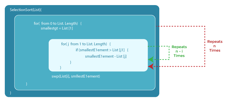
This results in a geometric total, and with basic high-school arithmetic, we can see that the inner loop will repeat 1+2... + n times, which equals n(n-1)/2 times. If we increase this by n²/2-n/2, we get n²/2-n/2.

When we compute large O notation, we just consider the dominating terms and ignore the coefficients. As a result, we choose n2 as our ultimate large O. We express it as O(n2), which is called "Big O squared" once more.

Big O notation's Formal Definition

Don't the numbers expand rather quickly afterwards for exponential growth? The same reasoning applies to computer algorithms. If the needed effort to complete a task grows exponentially with respect to the input size, it might become tremendously difficult.

The square of 64 is now 4096. If you multiply that figure by 264, it will be lost outside the meaningful digits. As a result, when we look at the growth rate, we just consider the prominent variables. And, because we want to study the growth with regard to the input size, the coefficients that just multiply the number rather than expanding with the input size are useless.

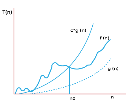
The formal definition of Big O is as follows:

• Big-Oh is about finding an asymptotic upper bound.
• Formal definition of Big-Oh:

f(N) = O(g(N)), if there exists positive constants c, N₀such that

f(N) ≤ c . g(N) for all N ≥ N₀

• We are concerned with how f grows when N is large
  • Not concerned with small N or constant factors
• Lingo: “ f(N) grows no faster than g(N)”

When performing a mathematical proof, the formal definition comes in handy. The temporal complexity of selection sort, for example, can be characterised by the function f(n) = n²/2-n/2, as stated in the preceding section.

If we let our function g(n) be n², we can discover a constant c = 1 and a N₀ = 0, and N² will always be bigger than N²/2-N/2 as long as N > N₀. We can readily demonstrate this by subtracting N²/2 from both functions, and we can show that N²/2 > -N/2 is true for N > 0. As a result, we may conclude that f(n) = O(n2), which is "large O squared" in the other selection sort.

You may have detected a tiny trick here. That is, if you make g(n) grow very quickly, far faster than anything else, O(g(n)) will always be large enough. For example, for every polynomial function, you can always be correct in declaring that it is O(2n), because 2n will ultimately surpass any polynomial.

You are correct mathematically, however when we talk about Big O, we want to know the function's tight bound. As you go through the next part, you will have a better understanding of this.

But before we continue, let's put your knowledge to the test with the following question. The solution will be found in later sections, so it will not be a waste of time.

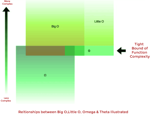
Big O, Little O, Omega & Theta

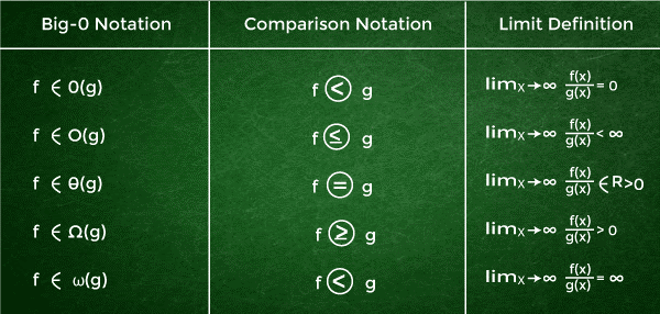
• Big O: “f(n) is O(g(n))” iff for some constants c and N0, f(N) ≤ cg(N) for all N > N0
• Omega: “f(n) is Ω(g(n))” iff for some constants c and N0, f(N) ≥ cg(N) for all N > N0
• Theta: “f(n) is θ(g(n))” iff f(n) is O(g(n)) and f(n) is Ω(g(n))
• Little O: “f(n) is o(g(n))” iff f(n) is O(g(n)) and f(n) is not θ(g(n))

To put it simply:

• Big O (O()): Big O (O()) denotes the complexity's upper bound.
• Omega (Ω()): The lowest bound of complexity is described by Omega (Ω()).
• Theta (θ()): Theta (θ()) expresses the complexity's precise bound.
• Little O (o()): The upper bound, omitting the precise bound, is described by Little O (o()).

The function g(n) = n2 + 3n, for example, is O(n³), O(n⁴), θ(n²) and Ω(n). However, you are correct if you state it is Ω (n²) or O(n²).

In general, when we talk about Big O, we really mean Theta. When you offer an upper bound that is far bigger than the scope of the research, it becomes rather useless. This is analogous to solving inequalities by placing on the bigger side, which usually always results in a correct answer.

Comparison of the Complexity of Typical Big Os

When attempting to determine the Big O for a certain function g(n), we only consider the function's dominating term. The dominating phrase is the one that increases the most quickly.

For example, n² grows faster than n, therefore if we have g(n) = n² + 5n + 6, it will be large O(n²). If you've ever taken calculus, you'll recognise this as a shortcut for calculating limits for fractional polynomials, where you only worry about the dominant term for numerators and denominators in the end.

There are several principles that govern which function increases quicker than others.

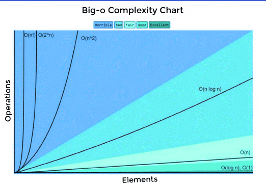
1. O(1) has the least amount of complexity.

If you can build an algorithm to solve the issue in O(1), you are probably at your best. This is sometimes referred to as "constant time." When the complexity of a scenario exceeds O(1), we can examine it by locating its O(1/g(n)) counterpart. O(1/n), for example, is more complicated than O(1/n²).

2. O(log(n)) is more complicated than O(1) but less so than polynomials.

Because difficulty is typically associated with divide and conquer algorithms, O(log(n)) is an useful complexity to aim for while developing sorting algorithms. Because the square root function is a polynomial with an exponent of 0.5, O(log(n)) is less difficult than O(n).

3. As the exponent grows, so does the complexity of polynomials.

O(n⁵), for example, is more complicated than O(n⁴). We actually covered through quite a few instances of polynomials in the previous sections due to their simplicity.

4. As long as the coefficients are positive multiples of n, exponentials are more difficult than polynomials.

Although O(2ⁿ) is more complex than O(n⁹⁹), O(2ⁿ) is really less complex than O(1). We usually choose 2 as the basis for exponentials and logarithms since everything in computer science are binary, although exponents may be modified by altering the coefficients. If the base for logarithms is not provided, it is presumed to be 2.

5. Factorials are more complicated than exponentials.

If you're curious in the logic, search up the Gamma function, which is an analytic continuation of a factorial. A quick demonstration is that factorials and exponentials both have the same amount of multiplications, but the numbers multiplied rise for factorials while maintaining constant for exponentials.

6. Terms for multiplication

The complexity of multiplication will be more than the original, but no more than the equivalence of multiplying something more complicated. O(n * log(n)) is more complicated than O(n) but less complex than O(n2) since O(n²) = O(n * n) because n is more complex than log (n).

Complexity of Time and Space

So far, we've simply spoken about the temporal complexity of the algorithms. That is, we are only concerned with how long it takes the programme to perform the task. What is equally important is the amount of time it takes the application to perform the task. Because the space complexity is connected to how much memory the programme will require, it is also an essential aspect to consider.

Space complexity operates in the same way that time complexity does. Because it only keeps one minimum value and its index for comparison, selection sort has a space complexity of O(1), and the maximum space consumed does not rise with input size.

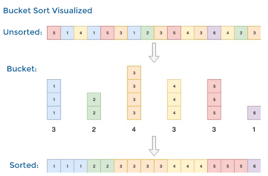
Some algorithms, such as bucket sort, have a space complexity of O(n) but a time complexity of O(n) (1). Bucket sort sorts the array by producing a sorted list of all the array's potential items, then incrementing the count everytime the element is found. Finally, the sorted array will consist of the sorted list components repeated by their counts.

Best, Average, Worst, Expected Complexity

The complexity may also be broken down into best case, worst case, average case, and expected case scenarios.

Take, for example, insertion sort. The insertion sort loops over all of the entries in the list. If the element is greater than the preceding element, the element is inserted backwards until it is larger than the previous element.

There will be no swap if the array is first sorted. The method will only traverse over the array once, resulting in a time complexity of O(n). As a result, the best-case time complexity of insertion sort is O(n). O(n) complexity is also known as linear complexity.

Sometimes an algorithm is simply unlucky. Quick sort, for example, must traverse the list in O(n) time if the items are sorted in the opposite order, but it sorts the array in O(n * log(n)) time on average. In general, when we analyse an algorithm's temporal complexity, we look at its worst-case performance. More on it, as well as a fast sort, will be detailed in the next part as you read.

The average case complexity describes the algorithm's predicted performance. Calculating the likelihood of each situation is sometimes required. Going into depth can become difficult, hence it is not covered in this article. A cheat sheet on the time and space complexity of common algorithms is provided below.

Why BigO isn't important?

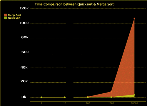
Given that the worst-case time complexity for quick sort is O(n2) but O(n * log(n)) for merge sort, merge sort should be quicker, right? You've probably figured that the answer is false. The algorithms are simply connected in such a manner that quick sort becomes "quick sort."

Take a look at this item to see what I mean. I created io. It compares the times for speedy and merge sorting. I've only tested it on arrays with lengths up to 10000, but as you can see, the time for merge sort climbs faster than the time for rapid sort. Despite the fact that rapid sort has a worst-case complexity of O(n2), the possibility of this happening is extremely low. When it comes to the gain in speed that fast sort has over merge sort, which is limited by the O(n * log(n)) complexity, quick sort outperforms merge sort on average.

I also created the graph below to compare the ratio of time they take, as it is difficult to discern them at lower numbers. And, as you can see, the percentage time required for rapid sort is falling.

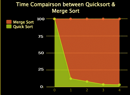
The lesson of the story is that Big O notation is nothing more than a mathematical analysis used to offer a reference on the resources spent by the method. In practise, the outcomes may differ. However, it is typically a good idea to strive to reduce the complexity of our algorithms until we reach a point where we know what we are doing.

How is complexity determined?

The time complexity is influenced by two factors: the amount of the input and the algorithm's solution. Here's a general formula for calculating complexity:

• List all of the code's fundamental operations.
• Count the number of times each is carried out.
• Add all of the counts together to generate an equation in terms of n.

Example:

Let's have a look at the code below and see how we can determine its complexity if the input size is equal to n:

#include <iostream>
using namespace std;


int main() {
  int sum = 0;
  for (int i=0;i<5;i++){
    sum = sum+i; 
  }
  cout << "Sum = " << sum;
  return 0;
}

Let's go over all of the statements and how many times they've been executed:

Operations	Executions
int sum = 0;	1
for ( int i = 0 ; i < 5; i ++ )	6
sum = sum + I;	5
cout << "Sum = " << sum;	1
return 0;	1

Calculations:

1+6+5+1+1

If we generalise this notation in terms of input size (n), we get the following expression:

• 1 + (n+1) + n + 1 + 1

After simplifying the above statement, the final time complexity is:

• 2n + 4

Follow these two steps to locate Big-O notation:

• Remove the leading constants.
• Ignore the words of lower order.

We may estimate the Big-O notation after completing the preceding two steps on the temporal complexity that we just calculated:

• 2n+4
• n+4
• n
• O(n)

The following is a list of Big-O complexity in increasing order:

Function	Name	Function	Name
O(1)	Constant	O(n2)	Quadratic
O(logn)	Logarithmic	O(n^3)	Cubic
O(log2n)	Log - Square	O(n^4)	Quartic
O(√n)	Root-n	O(2^n)	Exponential
O(n)	Linear	O(e^n)	Exponential
O(nlogn)	Linearithmic	O(n!)	O(n!)