Heap Sort vs Merge Sort

In this article, we are going to discuss the Heap Sort, Merge sort and the difference between them.

What is Heap Sort?

Heap – A heap is an abstract data type categorised into max-heap and min-heap. For all nodes in a heap, if the root node is greater than its children, it is referred to as the max-heap; if the root node is smaller than its children, it is referred to as the min-heap.

Heap Sort - A heap sort is also based on the comparison and selection method. It considers the given array as a heap, converts it into max-heap or min-heap, and then sorts the array by selecting and eliminating.

The pseudo-code of the functions involved in the heap sort is given below:

Heap Sort (Int A[], n)
{
Heap_size = n;
Build_max_heap(A, Heap_size);
For i = n-1 down to 2
{
Swap(A[1] and A[i];
Heap_size = Heap_size – 1;
Build_max_heap(A, Heap_size);
}
}


Build_max_heap(A, Heap_size)
{
For i = Heap_size/2 down to 1
{
Max_heapify(A, i);
}
}


Max_heapify(A, i)
{
L = Left(i) // Finding the left child
R = Right(i) // Finding the right child
Largest = i
If (L <= Heap_Size(A) and A[L] > A[Largest])
Largest = L
If (R <= Heap_Size(A) and A[R] > A[Largest]
Largest = R
If (Largest != i)
{
Swap (A[Largest] and A[i])
Max_heapify(A, Largest)
}
}

The heap sort involves three functions, the Max_heapify function places the value at the ith index at its correct position in a heap, and the Build_max_heap function converts the given array into a max-heap. The Heap_sort function calls the necessary function until the array gets sorted.

Click on the given link for the implementation of the heap sort https://www.tutorialandexample.com/heap-sort

Let us sort an array using the Heap sort to get its whole idea and steps involved.

Consider an array, A[] = {14, 28, 12, 36, 5, 18, 9} of size = 7. When we call the heap sort function, it further calls the Build_max_heap function and the Build_max_heap function calls the Max_heapify function. After completing the first Build_max_heap function, we get a max heap.

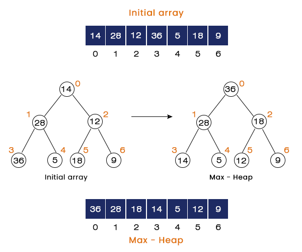
Now, we have a max-heap of height = 3.

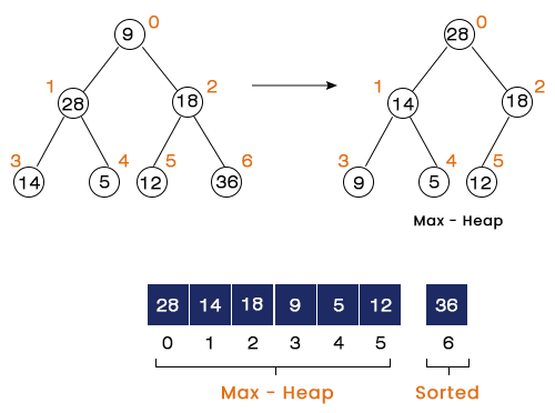
Pass 1 – Swap (36 and 9). After swapping, the largest value reaches the last index at its correct position. Now, call the max-heapify at index = 0 to convert it into a max-heap with the number of elements = 6.

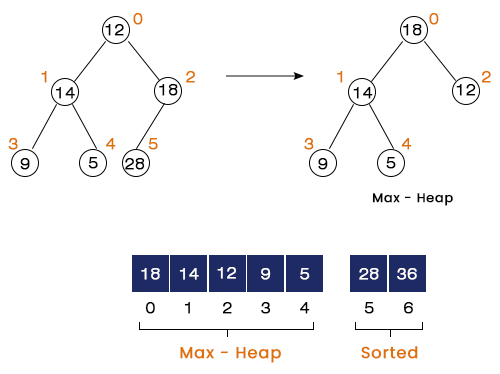
Pass 2 – Swap (28 and 12). After swapping, 28 reaches its correct position at index = 5. We again call the max-heapify at index = 0 to convert it into a max-heap with the number of elements = 5.

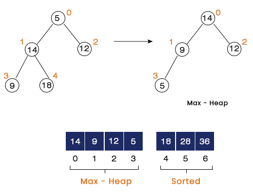
Pass 3 - Swap (18 and 5). After swapping, 18 reaches its correct position at index = 4. We again call the max-heapify at index = 0 to convert the remaining array into a max-heap with the number of elements = 4.

We continue the same procedure for the other passes.

Pass 4 – Swap (14 and 5). After swapping, 14 reaches its correct position at index = 3.

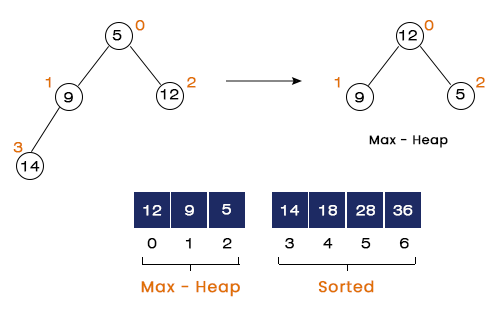
Pass 5 - Swap (12 and 5). After swapping, 12 reaches its correct position at index = 2.

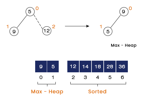
Pass 6 - Swap (9 and 5). After swapping, 9 and 5 reach their correct positions at index = 1 and 0, respectively.

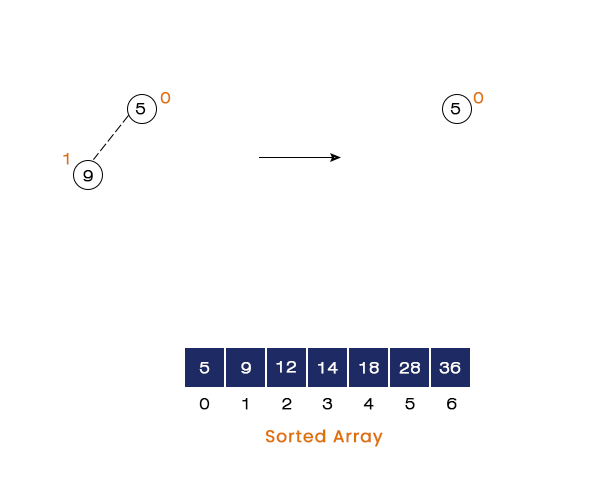
After complete execution of the heap sort function, we get a sorted array as the output.

Let’s move to the next sorting technique Merge Sort

What is Merge Sort?

Merge Sort – The merge sort is a divide and conquer technique that divides a bigger problem into two sub-problems, and each sub-problem is further addressed separately. The out of the program is formed by combining all the results of each sub-problems.

The Pseudo-code of the Merger sort function is given below:

Merge_sort (A, L, U)
{
If(L<U)
{
M = (L + U)/2
Merge_sort (A, L, M);
Merger_sort (A, M + 1, L);
Merge (A, L, M, U);
}
} // L -> Lower Bound, M -> Middle Index, and U -> Upper bound


Merge (A, L, M, U)
{
N1 = M – L + 1;
N2 = U – M;
Create New Array A1[0 to N1] and A2[0 to N2]
For i = 0 to N1
A1[i] = A[ L + i]
For j = 0 to N2
A2[j] = A[M + j]
A1[N1] = Infinity
A2[N2] = Infinity
i = 0;
j = 0;


For k = L to U
If(A1[i] <= A2[j])
{
A[k] = A1[i];
i = i + 1;
}
Else
{
A[k] = A2[j];
j = j + 1;
}
}

The Merge sort function divides the problems into two subproblems of size L to M and M+1 to U, and the Merge function merges the two subproblems into one. In the Merge function, we store infinity at the last index of the newly created arrays A1 and A2. The idea is if somehow one array becomes empty, the elements of the other array are compared with the infinity and placed in array A.

Dividing and Merging Method

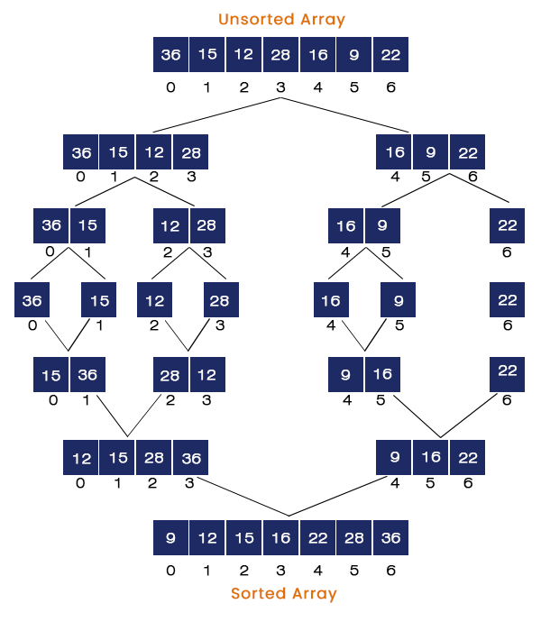
An array passed to the merge sort function is divided from the index 0 to n/2 and (n/2 + 1) to n-1, where n is the number of elements in the array. A1[0 to n/2] and A2[n/2 + 1 to n-1], these two problems are further divided until the size of the sub-problem becomes equal to 1. After that, the Merge function merges the subproblems and places all the elements in the right order. The same is shown in the given figure.

Let us take understand the above idea through an example:

Consider an unsorted array a[] = {36, 15, 12, 28, 16, 9, 22} of size equal to 7. The steps included in sorting the given array are listed below:

Step 1– In the first step, the array of size = 7 is divided into two sub-problems of sizes 4 and 3. We have two Merge sort function calls Merge_sort(A, 0, 3) and Merge_sort(A, 4, 6)and one Merge function call Merge(A, 0, 3, 6). The first Merge_Sort function is solved in the next step, and the rest of the statements are stored in the stack.

Step 2 – Merge_sort(A, 0, 3) is called in the second step. Now, we again have two merge sort function calls Merge_sort(A, 0, 1) and Merge_sort(A, 2, 3) and one Merge function call Merge(A, 0, 1, 3). Merge_sort(A, 0, 1) is called first, and the rest of the function calls are stored in the stack.

Step 3 – The Merge_sort(A, 0, 1) is called. We have Merge_sort(A, 0, 0), Merge(A, 1, 1) and Merge(A, 0, 0, 1). For the first time, we have two merge sort function calls where L and U are equal. Now, the subproblems size is 1; hence Merge function is called for the First time.

Step 4 – The Merge(A, 0, 0, 1) is called. It merges the elements present at the index 0 and 1 in the right order. 15 is stored at index 0, and 36 is stored at index 1.

Step 5 – Like above, other function calls are made and executed. Here, Merge_sort(A, 2, 3) is called. It is further divided and Merged by the program. For this function call, 12 and 28 are placed at the index = 2 and 3, respectively.

Step 6 – The Merge(A, 0, 1, 3) is called and executed by the program. The half of the array gets sorted in this step. The elements of Array A from the index 0 to 3 are placed in a sorted manner. A[0 -> 3] = {12, 15, 28, 36}.

Step 7 – Till here, we have completed half of the program. Merge_sort(A, 4, 6) is called and executed in this step. We further call Merge_sort(A, 4, 5), Merge_sort(A, 6, 6), and Merge(A, 4, 5, 6).

Step 8 – The Merge_sort(A, 4, 5) is called. We divide it into two subproblems of sizes 1 and merge them afterwards. Now, we call the Merge(A, 4, 5, 6). After executing this merge call, we get A[4 -> 6} = {9, 16, 22}.

Step 9 – In the last step, We merge A[0 -> 3] = {12, 15, 28, 36} and A[4 -> 6} = {9, 16, 22}. After merging them, we get A[0 -> 6] = {9, 12, 15, 16, 22, 28, 36}.

Difference between Heap Sort and Merge Sort:

The main difference between Heap Sort and Merge Sort are listed below in the table:

Heap Sort	Merge Sort
The idea is to convert the given array into a heap and then sort the array by placing the root element at the last index and repeating the same process for the remaining n-1 elements.	The idea is to divide a problem into two subproblems and merge the element of these two subproblems into one. Each subproblem is divided into two subproblems until their size becomes equal to 1.
Time Complexities: Worst Case: T(n) = O(nlogn) Average Case: T(n) = O(nlogn) Best Case: T(n) = O(nlogn)	Time Complexities: Worst Case: T(n) = O(nlogn) Average Case: T(n) = O(nlogn) Best Case: T(n) = O(nlogn)
The space complexity of the heap sort is O(1). It does not require any extra space.	The space complexity of the Merge sort is O(n). It requires extra space.
The heap sort is slower than the Merge Sort.	The Merge Sort runs slow for arrays of small sizes and faster for large ones.
It is an unstable sorting algorithm. The order of the identical elements does not remain preserved.	It is a stable sorting algorithm. The order of identical elements remains preserved.
It uses the idea of Binary heaps.	It uses dividing, comparing and merging ideas.
The heap sort has the time complexity as a ‘divide and conquer’ method, but it’s similar to the selection sort.	It is a ‘divide and conquer’ sorting method.