Quick Sort vs Merge Sort

In this article, we will take an overview of Quick Sort and Merge Sort and then discuss the differences between them.

What is Quick Sort?

Quick Sort – The idea behind the quick sort is to select a random pivot element and place all the elements smaller than the pivot on its left side and larger elements on the right side and repeat the same process for the left and right sides of the pivot element. It follows the ‘divide and conquer’ technique and makes nlogn comparisons to sort the elements of an array.

How is a pivot element selected?

The performance of the quick sort depends on selecting a good pivot element. However, it isn’t very easy to determine the best pivot element. The left, right, or middle elements are generally chosen as the pivot elements; sometimes, any random element can be selected as the pivot element.

Dividing / Partition technique:

As soon as the pivot element is selected, the array is divided into two parts/subarrays. All the values smaller than the pivot element are stored on the left side of the pivot element, and all the elements larger than the pivot element are stored on the right of the pivot element. We perform the quick sort on the left and right sub-arrays separately until only one element remains in the sub-arrays.

The pseudo-code of the recursive quick sort algorithm is given below:

Quick_Sort (A, l, r)
{
	If (l < r)
	{
		q = partition (A, l, r)
		Quick_Sort (A, l, q - 1)
		Quick_Sort (A, q + 1, r)
	}
}

Pseudo-code of the partition function:

Partition (A, l, r)
{
	Pivot = A[r]
	i = l -1
	for j = 0 to r - 1
	{
		If (A[j] <= Pivot)
		{
			i = i + 1
			Swap (A[i] and A[j])
		}
	}
	Swap (A[i + 1] and A[r])
	Return i + 1 // Index of the pivot element
}

Let us now understand the steps involved in sorting an array using the Quick Sort:

Consider an array A[] = {12, 45, 23, 3, 41, 9, 33, 25} of size = 8. The steps involved in sorting the given array using the Quick sort are explained below:

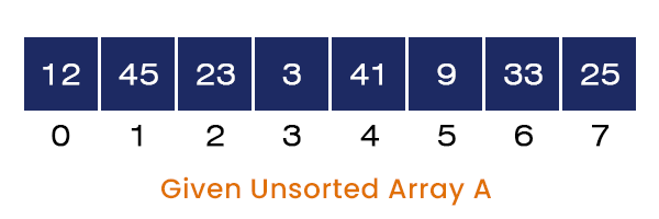
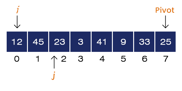
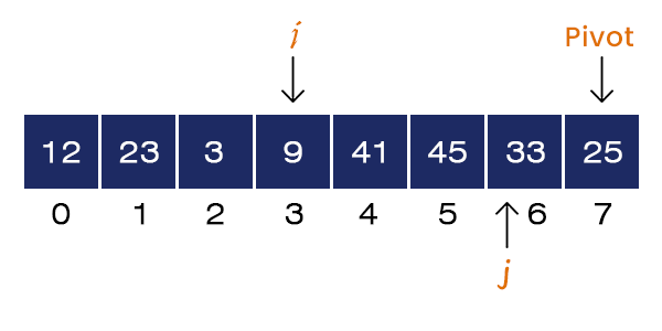
When we call the quick sort function, it first calls the partition function with the same parameters, Partition (A, 0, 7). We first select the rightmost element as the pivot element, Pivot = A[7] = 25. We set the value of i = l - 1 = -1 and start the for loop from the left side, j = 0.

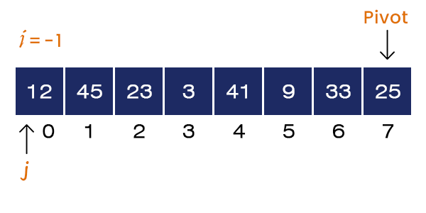
Here, A[j = 0] = 12 < Pivot. If-condition is satisfied. We set i = i + 1 = 0. Here, i and j are equal to 0, swapping does not affect the array.

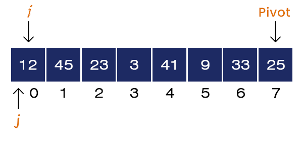
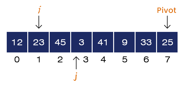
Now, j = 1 and A[j] = 45 > Pivot. If-condition is not satisfied, no swapping occurs. We increment the value of j = 2.

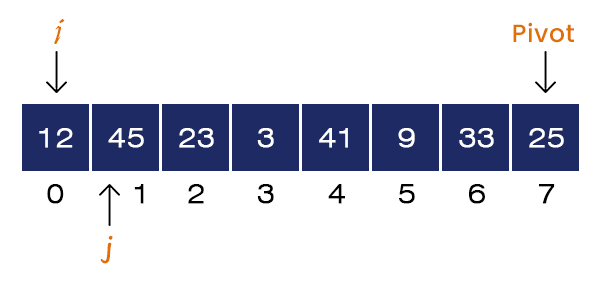
Now, j = 2 and A[j] = 23 < pivot. If-condition is satisfied, we set i = i + 1 = 1 and Swap a[1] = 45 and a[2] = 23. We increment the value of j = 3.

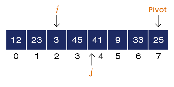
Now j = 3 and A[j] = 3 < pivot. If-condition is satisfied, we set i = i + 1 = 2 and Swap a[2] = 45 and a[3] = 3. We increment the value of j = 4.

Now, j = 4 and A[j] = 41 > Pivot. If-condition is not satisfied, no swapping occurs. We increment the value of j = 5.

Now j = 5 and A[j] = 9 < pivot. If-condition is satisfied, we set i = i + 1 = 3 and Swap a[3] = 45 and a[5] = 9. We increment the value of j = 6.

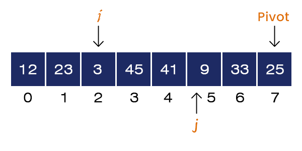
Now, j = 6 and A[j] = 33 > Pivot. If-condition is not satisfied, no swapping occurs. For loops terminates.

Now, we swap A[i+1] = 45 and A[r] = 25. After swapping, the pivot element is placed at its correct position.

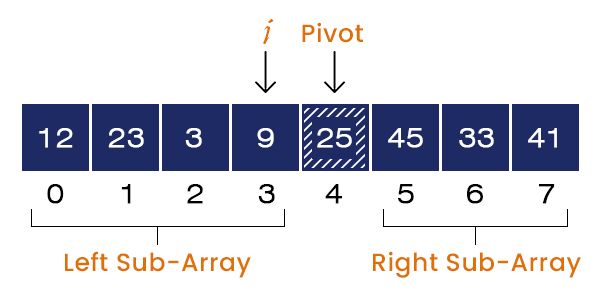
We have unsorted left and right subarrays. i + 1 = 4, the index of the pivot element is returned to the quick sort function.

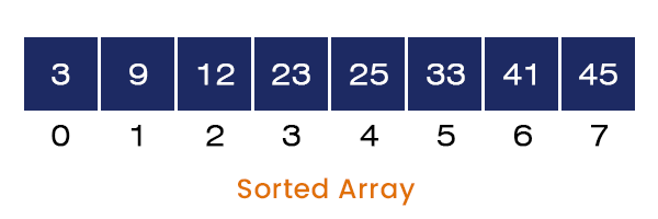
We perform the same steps on the left and the right subarrays. After that, we get a sorted array as the program’s output.

Now, let us discuss the idea of Merge Sort:

What is the merge sort?

The merge sort uses the Divide and Conquer technique to sort a list of elements. It divides a problem into two subproblems until the size of each subproblem becomes equal to 1 and starts merging all the subproblems by comparing and placing all the elements in their correct order.

The pseudo-code of the Recursive Merge sort function:

Merge_sort (A, L, U)
{
	If(L<U)
	{	
		M = (L + U)/2
		Merge_sort (A, L, M);
		Merger_sort (A, M + 1, L);
		Merge (A, L, M, U);
	}
} // L -> Lower Bound, M -> Middle Index, and U -> Upper bound

The Merge sort function recursively calls itself until the subproblem’s size is not equal to 1 and calls the merge function after that.

The pseudo-code of the Merge Function:

Merge (A, L, M, U)
{
	N1 = M – L + 1;
	N2 = U – M;
	Create New Array A1[0 to N1] and A2[0 to N2]


	For i = 0 to N1
		A1[i] = A[ L + i]


	For j = 0 to N2
		A2[j] = A[M + j]


	A1[N1] = Infinity
	A2[N2] = Infinity


	i = 0;
	j = 0;


	For k = L to U
	{
		If(A1[i] <= A2[j])
		{
			A[k] = A1[i];	
			i = i + 1;
		}


		Else
		{
			A[k] = A2[j];
			j = j + 1;
		}
	}
}

The Merge function merges the array from the index L to U with the middle index M by storing the elements from L to M into a newly created array (A1) and from M + 1 to U into another newly created array (A2) and comparing each element with one another.

To understand the above idea of merge sort, let us take an example and perform merge sort on it:

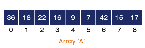
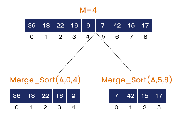
Consider an array A[] = {36, 18, 22, 16, 9, 7, 42, 15, 17} having nine elements in it. The steps involved in sorting the above array are listed below:

• Calling Merge_Sort (A, 0, 8)
  M = (L + U) / 2 = 4, It calls Merge_Sort (A, 0, 4), Merge_Sort (A, 5, 8) and Merge (A, 0, 4, 8). The Merge_Sort (A, 0, 4) is called first and the rest of the function calls will go to the stack.

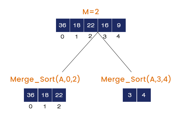
• Calling Merge_Sort (A, 0, 4)
  M = (0 + 4) / 2 = 2, It calls Merge_Sort (A, 0, 2), Merge_Sort (A, 3, 4) and Merge (A, 0, 2, 4). The Merge_Sort (A, 0, 2) is called and the rest of the function calls will go to the stack.

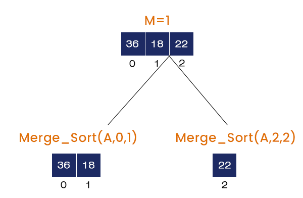
• Calling Merge_Sort (A, 0, 2)
  M = (0 + 2) / 2 = 1, It calls Merge_Sort (A, 0, 1), Merge_Sort (A, 2, 2), and Merge (A, 0, 1, 2). The Merge_Sort (A, 0, 1) is called and the rest of the function calls will go the stack.

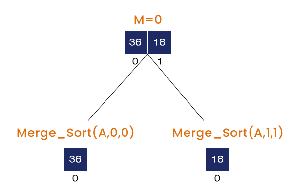
• Calling Merge_Sort (A, 0, 1)
  M = (0 + 1) / 2 = 0, It calls Merge_Sort (A, 0, 0), Merge_Sort (A, 1, 1), and Merge (A, 0, 1, 1). Here, when the first two merge sort function calls are called nothing is executed and finally at the last Merge (A, 0, 1, 1) is called.

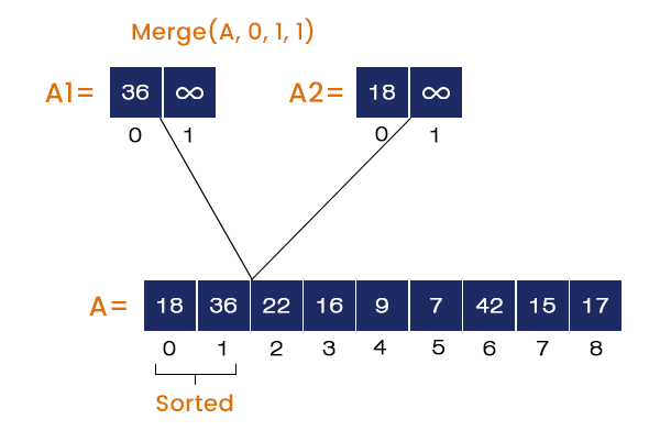
• Calling Merge (A, 0, 1, 1)
  The value = 36 at the index = 0 is stored in array A1, and the value = 18 at the index = 1 is stored in array A2. The merge function compares the elements in A1 and A2 and stores them in array A in ascending order. So, 18 is placed at index = 0 and 36 is placed at index = 1 in A.

Now, we have Merge_sort (A, 2, 2) at the top of the stack. But here, L = 2 is equal to U = 2, so nothing will happen. We will pop the next element from the stack and start executing.

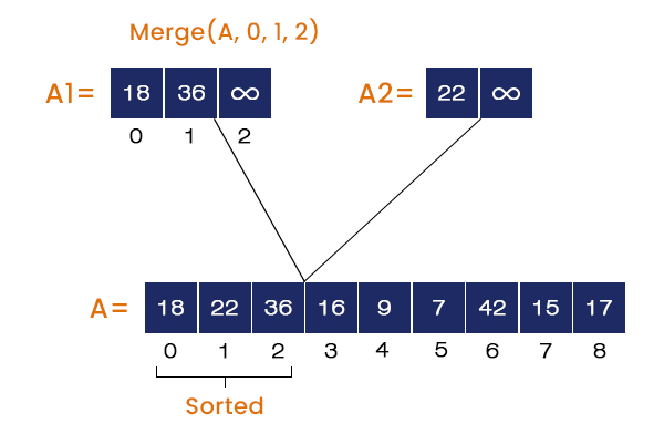
• Calling Merge (A, 0, 1, 2)
  The elements from the index 0 to 1 are stored in array A1, and the element at index = 2 is stored in array A2. The merge function compares all the elements of both A1 and A2 and stores the element in A in ascending order. So, 18, 22, and 36 are stored at index = 0, 1, 2 respectively in A.

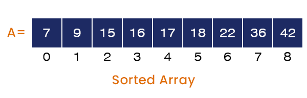
We will pop all the stack elements (Function Calls) and execute them one by one. We repeat the same process for all the function calls, and at the end of the program, we get a sorted array as the output, which would be A[] = {7, 9, 15, 16, 17, 18, 22, 36, 42}.

Now let’s move to the next topic differences between Quick Sort and Merge Sort:

The Quick sort and Merge sort both follow the ‘Divide and Conquer’ principle, but there are some fundamental differences between the idea behind these sorting techniques. Some of the main differences are listed below in the table:

Quick Sort	Merge Sort
The idea is to select a random pivot element and place all the elements smaller than the pivot on its left side and all the elements larger than the pivot on its right side in the array. After that, repeat the same process for the left and right subarrays separately.	The idea is to divide a given array into two subarrays from the middle and repeat the same process for the subarrays too until the subarray size becomes equal to 1 and merge all the elements by comparing with the help of newly created arrays in the correct order.
Its best and average time complexities are O(nlogn), but in the worst case, it becomes equal to O(n^2). This is when it selects the smallest or largest as the pivot element every time.	Its best, average, and worst-case time complexities are O(nlogn).
In the worst case, it behaves like the subtract and conquer technique. We can conclude that it depends on the content.	It does not depend on the content rather; it depends on the structure. It always behaves like the ‘divide and conquer’ technique.
Its space complexity is O(1) as it requires no extra space.	Its space complexity, in the worst case, reaches the O(n).
It is an internal sorting technique.	It is an external sorting technique.
It is not a stable sorting technique. The order of identical elements does not remain preserved.	It is a stable sorting technique. The order of identical elements remains preserved.
It is less efficient compared to merge sort.	More efficient than the quick sort.