Bubble Sort vs Merge Sort
In this article, we are going to compare two sorting techniques, Bubble sort and Merge Sort. In starting, we will first discuss the idea of sorting an array using bubble sort and merge sort both, and later on, we will discuss their differences.
Let’s start the discussion with the bubble sort.
Q. Discuss the idea of bubble sort through an example:
Bubble sort - The bubble sort is a ‘subtract and conquer’ based sorting technique. In which it continuously compares all the elements and places all the elements in their right order. It is called bubble sort because it only compares two adjacent elements referred to as the bubble at any instant.
On each complete iteration of the internal for loop, the largest element is placed at the last index of the unsorted part of the array.
The pseudo-code of the Bubble Sort Function:
1. Bubble Sort (A, N)
2.	For I = 1 to N - 1
3.		For J = 0 to N - I – 1
4.			If A[J] > A[J + 1]
5.				Swap (A[J], A[J + 1])
//N – Number of elements in the array A.
As we can see in the above pseudo-code of the bubble sort function, the internal for loop begins at index = 0 and ends at index N – I – 1 and the external for loop begins at index = 0 and ends at index N – 1.
Now let us understand the idea of sorting an array using the bubble sort:
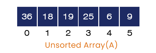
Consider an array A[] = {36, 18, 19, 25, 6, 9} with six elements in it; the steps involved and stages of the array on each stage are listed below:
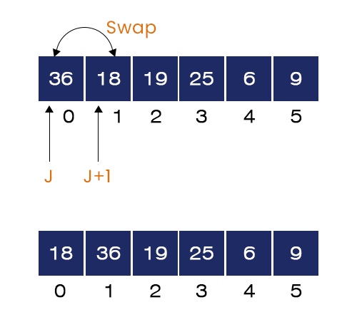
1.First pass of the external for loop – I begins at index = 0, and J begins at index = 0 and ends at index = 6 – 1 – 1 = 4.
- When J = 0, the element at index j is A[j] = 36 and element at index j+1 is A[j + 1] = 18. Here, A[J] > A[J+1] hence, the if-condition is true. We swap 36 and 18 and go to the next iteration.
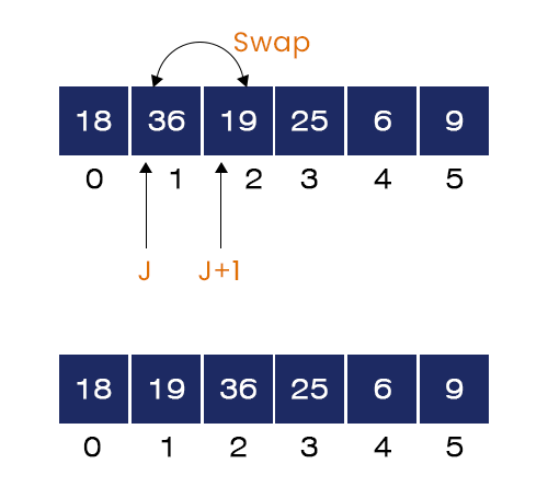
- When J = 1, the element at index j is A[j] = 36 and element at index j+1 is A[j + 1] = 19. Here, A[J] > A[J+1] hence, the if-condition is true. We swap 36 and 19 and go to the next iteration.
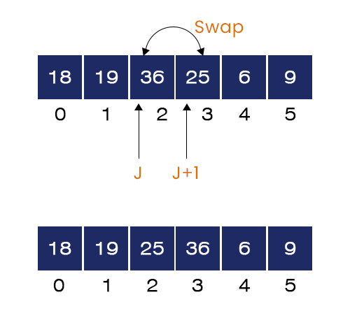
- When J = 2. Here, A[J] = 36 and A[J+1] = 25. A[J] > A[J+1] hence, the if-condition is true. We swap 36 and 25 and go to the next iteration.
- When J = 3. Here, A[J] = 36 and A[J+1] = 6. A[J] > A[J+1] hence, the if-condition is satisfied. We swap 36 and 6 and go to the next iteration.
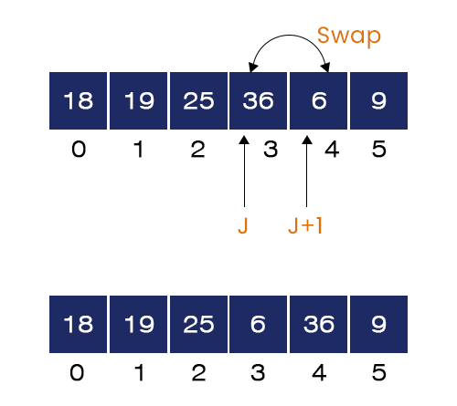
- When J = 4. Here, A[J] = 36 and A[J+1] = 9. A[J] > A[J+1] hence, the if-condition is satisfied. We swap 36 and 9 and go to the next iteration.
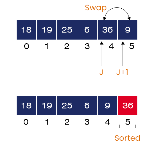
We can see that the largest element = 36 is now placed at its correct position. The first cycle of the internal for-loop ends here.
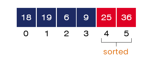
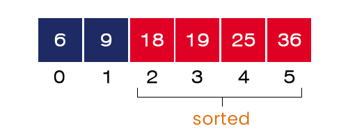
2. Second pass of the external for-loop - As we have observed from the above pass, on each complete execution of the internal for loop, the largest element goes at the end of the unsorted part of the array. So, in this iteration after completing all the steps of the internal for-loop, the second largest element = 25 gets placed at index = 4. The same is shown in the figure below:
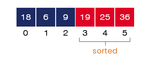
3. Third Pass – In this pass, after completing the execution of the internal for-loop, the third largest element = 19 gets placed at index = 3.
4. Fourth Pass – After completing the execution of the internal for loop, the fourth largest element = 18 gets placed at index = 2.
5. Fifth Pass – At the end of the execution of the internal for-loop, the fifth largest element = 9 gets placed at index = 1, and the smallest element takes its position in the array at index = 0.
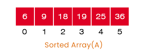
After completing all the passes, we get the required sorted array as the output of the program without any error.
Now, we are ready to understand the idea of merge sort.
Q. Discuss the idea of merge sort through an example.
Merge Sort – The merge sort uses the ‘divide and conquer’ technique to sort elements. The idea of merge sort is to divide a big problem into two subproblems until the size of the subproblems equals 1. After that, it starts merging all the subproblems one by one by comparing the elements and placing them in their right order.
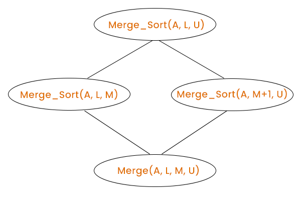
Dividing Method – Suppose an array with nine elements is passed to the merge sort function. It first calculates the Middle index and divides the array into two subarrays from the middle index. Let’s say the middle index is M; so, the indexing of one subarray would be L to M, and the indexing of another subarray would be M+1 to U, where L and U are the lower and upper bounds of the array. It will recursively further divide these two subproblems into respective subproblems.
Merging Method – The merging method is based on the idea of merging two sorted arrays. As we know, an array with an element is a sorted array. When the subproblem size becomes equal to 1, it starts merging them in ascending or descending order as programmed until all the elements are not placed in sorted order.
Let us see the pseudo-code of the merger sort algorithm:
The pseudo-code of the merge sort function:
1. Merge Sort (A, L, U)
2.	If (L < U)
3.		M = (L + U) / 2
4.		Merge Sort (A, L, M);
5.		Merger Sort (A, M + 1, L);
6.		Merge (A, L, M, U);
// L -> Lower Bound, M -> Middle Index, and U -> Upper bound
The pseudo-code of the merge function:
1. Merge (A, L, M, U)
2.	N1 = M – L + 1;
3.	N2 = U – M;
4.	Create New Array A1[0 to N1] and A2[0 to N2]


5.	For i = 0 to N1
6.		A1[I] = A[ L + I]


7.	For j = 0 to N2
8.		A2[J] = A[M + J]


9.	A1[N1] = Infinity
10.	A2[N2] = Infinity


11.	I = 0;
12.	J = 0;


13.	For K = L to U
14.		If(A1[I] <= A2[J])
15.			A[K] = A1[I];
16.			I = I + 1;


17.		Else
18.			A[k] = A2[J];
19.			J = J + 1;
The whole idea of merge sort is based on the recursion. So, it is necessary to understand how these function calls are made.
Let us understand the above idea through an example:
Consider an array A[] = {14, 12, 9, 25, 5} with five elements is passed to the Merge sort function.
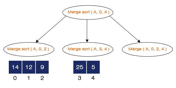
Step 1 – Merge Sort (A, 0, 4) is called.
We first calculate the middle Index, M = (0 + 4) / 2 = 2. Now, it calls the Merge Sort (A, 0, 2), Merge Sort (A, 3, 4) and Merge (A, 0, 2, 4). Merge Sort (A, 0, 2) is called first, and the rest of the function calls are pushed into the stack.
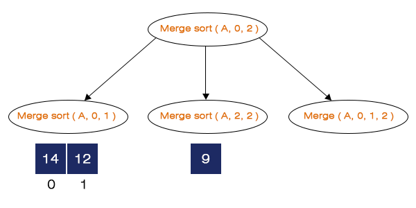
Step 2 – Merge Sort (A, 0, 2) is called.
Calculating the middle index, M = (0 + 2) / 2 = 1. It calls the Merge sort (A, 0, 1), Merge Sort (A, 2, 2) and Merge (A, 0, 1, 2). Here, the Merge sort (A, 0, 1) is called first, and other function calls are pushed into the stack.
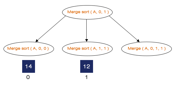
Step 3 - Merge sort (A, 0, 1) is called.
Calculating the middle index, M = (0 + 1) / 2 = 0. It calls Merge sort (A, 0, 0), Merge Sort (A, 1, 1) and Merge (A, 0, 1, 1). Here, when we call the Merge sort (A, 0, 0) for that if-condition fails and it will make no other function calls, and when we call the next function call, which is Sort (A, 1, 1), if-condition is not satisfied. Hence, it will also make no function calls. Now, we call the Merge (A, 0, 1, 1).
Step 4 – Merge (A, 0, 1, 1) is called.
It will create two new arrays, A1 and A2 of size N1 = 2 and N2 = 2, and store the elements of A in them. A1 stores the element present at index = 0, and A2 stores the element present at index = 1. The same is shown in the figure below:
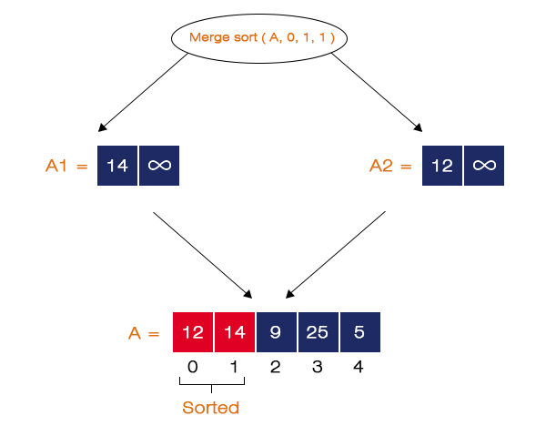
It will compare the elements from A1 and A2 and store them in array A in ascending order. Here, 14 > 12, so 12 is stored at index 0, and 14 is stored at index 1 in A.
Now, the next function call we have is Merge Sort (A, 2, 2). When it is called, the if-condition is satisfied. So, it will not call any other functions. Now, the next function call we have is Merge (A, 0, 1, 2).
Step 5 - Merge (A, 0, 1, 2) is called
It also creates two new arrays A1 and A2 of size N1 = 3 and N2 = 2 respectively. The elements of A from index 0 to 1 are stored in A1 and from 2 to 2 is stored in A2. The same is shown in the figure below:
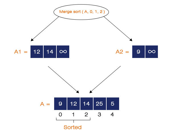
Now, it compares the elements of A1 and A2 and stores them in A in ascending order. And the elements from index zero to 2 of array A are now in the sorted sequence.
The same steps we follow for the Merge sort (A, 3, 4) function call and at the end it merges all the elements in ascending order same as above. The complete steps are shown in the figure below:
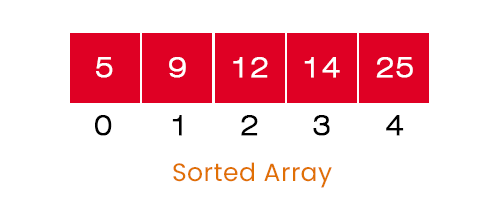
Now, the program terminates and we have a sorted array as the output of the merge sort algorithm.
Now, let us discuss what makes these sorting techniques differ from one another. Some of the main differences are listed below in the table:

| Bubble Sort |
Merge Sort | |||
| Definition | The idea is to compare the adjacent elements simultaneously and swaps them if they are not in the sorted sequence. | The idea is to divide a big problem into two sub-problems and merge the elements of the sub-problems in the sorted sequence with the help of some extra space. | ||
| Approach | It is based on the ‘subtract and conquer’ technique. | It is based on the ‘divide and conquer’ technique. | ||
Time complexity |
Best case | T(n) = O(n) | Best case | T(n) = O(n) |
| Average case |
T(n) = O(n^2) |
Average case |
T(n) = O(n^2) |
|
| Worst case | T(n) = O(n^2) | Worst case | T(n) = O(n^2) | |
| Best case comparison | In the best case, we pass a sorted array and it achieves the time complexity of the order of n, O(n). The flag version of it detects whether the array is already sorted or not in a single run of the internal for-loop. | Its time complexity does not change for any cases. We can say that it is a structure-dependent sorting technique. | ||
| Recurrence Relation | T(n) = T(n-1) + n | T(n) = 2T(n/2) + n | ||
| Stability | Stable | Stable | ||
| Efficiency | Less Efficient | More Efficient | ||
| Space Type | Internal – It does not require any extra space. | External – It requires extra space. | ||
| Method | It is based on the exchanging method. | It is based on the Merging method. | ||
| Size dependency | Performs well for small data. | Performs well for big data. | ||
| Speed | Slower | Faster | ||