Adjacency matrix program in C++ language
Introduction
A square matrix which is utilized for representing a finite graph is called an adjacency matrix.
A square matrix with dimensions of V x V represents the adjacency matrix of the graph. The graph G's vertex count is represented by the V. The V vertices on either side of this matrix are demonstrated. The adjacency matrix at the ith row along with the jth column will store 1 (or some number for the weighted graph) if the graph contains edges connecting i to j vertices; alternatively, it will continue to store 0. It is a technique for displaying the graph as a Boolean matrix made up of zeros and ones. The matrix's Boolean values shows the direct path links of two vertices. Adjacency lists and adjacency matrices are two ways to describe a graph. We express graphs in the adjacency matrix technique using the values '0' and '1'. For an undirected graph, let matrix[i][j] be the adjacency matrix. If a path exists from node 'i' to node 'j', then matrix[i][j] will equal 1, and matrix[j][i] will also equal 1. An adjacent matrix is consistently symmetric.
Complexity for adjacency matrix representation:
Creating the adjacency matrix with an O(n2) time complexity, considering the graph contains n vertices. In addition, the space complexity is O(n2). For graph, we must make a square matrix of n*n and then filling the matrix values with 0 and 1 in order to construct the adjacency matrix. We pay O(n2) space for it.
We must determine if an edge connects each pair (v(i), v(j)) of vertices in order to fill all of the values of the matrix. There are =
pairs of vertices in total for n vertices. For this reason, the matrix's construction has an O(n2) time complexity. Hence,
Time Complexity = O(n2 )
Space Complexity = O(n2)
Adjacency Matrix
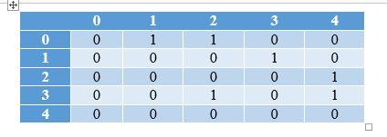
1. Input (Undirected Graph):
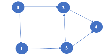
Output matrix:
| 0 | 1 | 2 | 3 | 4 | |
| 0 | 0 | 1 | 1 | 0 | 0 |
| 1 | 0 | 0 | 0 | 1 | 0 |
| 2 | 0 | 0 | 0 | 0 | 1 |
| 3 | 0 | 0 | 1 | 0 | 1 |
| 4 | 0 | 0 | 0 | 0 | 0 |
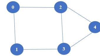
2. Input (Undirected Graph):
Output matrix:
| 0 | 1 | 2 | 3 | 4 | |
| 0 | 0 | 1 | 1 | 0 | 0 |
| 1 | 1 | 0 | 0 | 1 | 0 |
| 2 | 1 | 0 | 0 | 1 | 1 |
| 3 | 0 | 1 | 1 | 0 | 1 |
| 4 | 0 | 0 | 1 | 1 | 0 |
C++ program for adjacency matrix
#include <iostream>

using namespace std;

class Graphs

{

    private:

  bool** adj_Matrix;

  int Vertices;

   public:

  Graphs(int Vertices)

  {

    this->Vertices = Vertices;

    adj_Matrix = new bool*[Vertices];

    for (int i = 0; i < Vertices; i++)

    {

      adj_Matrix[i] = new bool[Vertices];

      for (int j = 0; j < Vertices; j++)

        adj_Matrix[i][j] = false;

    }

  }

  void adding_Edge(int i, int j)

  {

    adj_Matrix[i][j] = true;

    adj_Matrix[j][i] = true;

  }

  void removing_Edge(int i, int j)

  {

    adj_Matrix[i][j] = false;

    adj_Matrix[j][i] = false;

  }

  void toString()

  {

    for (int i = 0; i < Vertices; i++)

    {

      cout << i << " : ";

      for (int j = 0; j < Vertices; j++)

      {

        cout << adj_Matrix[i][j] << " ";

      }

      cout << "\n";

    }

  }

  ~Graphs()

  {

    for (int i = 0; i < Vertices; i++)

      delete[] adj_Matrix[i];

    delete[] adj_Matrix;

  }

};

int main()

{

  Graphs g(5);

  g.adding_Edge(0, 1);

  g.adding_Edge(0, 2);

  g.adding_Edge(1, 3);

  g.adding_Edge(2, 0);

  g.adding_Edge(2, 3);

  g.adding_Edge(2, 4);

  g.adding_Edge(3, 4);

  g.toString();

}
Output:
Advantages of adjacency matrix
- Basic constant time functions are very efficient when it comes to adding, deleting, and determining if there exists an edge between vertex i and vertex j.
- In cases when the graph is complex and has a high number of edges, the best option would be an adjacency matrix. We can use data structures for the sparse matrices to represent the graph in spite of an adjacency matrix are sparse.
- However, the application of matrices yields the more benefit. Recent hardware developments allow us to use the GPU for even more costly matrix computations.
- We can acquire vital information about the structure of the graph and the connections between its vertices by executing operations on the neighbouring matrix.
Disadvantages of adjacency matrix
- The adjacency matrix requires a lot of memory due to its VxV space need. Since most graphs seen in the real world have a limited number of connections, adjacency lists are often a preferable option for most purposes.
- While the adjacency matrix format makes fundamental operations simple, more complex operations such as inEdges and outEdges are costly.
Applications of adjacency matrix
- Navigation tasks
- Creating routing tables in any network
Conclusion
An adjacency matrix indicates a 2D array with a dimension of V x V, where V is the graph's vertex count. The implementation of adjacency matrix in C++ in shown above for the undirected graph. In the case of directed graph matrix[i][j] = 1 is assigned when there is an edge from vertex i to vertex j apart from this implementation of code is same for both the directed and undirected graph.