Cross Entropy in Python

Introduction

Cross-entropy loss is frequently combined with the softmax function. Determine the total entropy among the distributions or the cross-entropy, which is the difference between two probability distributions. For the purpose of classification model optimization, cross-entropy can be employed as a loss function.

What is Cross Entropy Loss?

A classification model that classifies the data by predicting the probability (value ranging from zero and one) of whether the data belongs to one class or another is trained using the cross-entropy loss function, an optimization function. The cross-entropy loss value is high if the projected probability of class differs significantly from the actual class label (zero or one).

The cross-entropy loss will be lower if the projected probability of the class is close to the class label (0 or 1). For models with softmax output, the loss function that is most frequently used is cross-entropy loss. Remember that multinomial logistic regression uses the softmax function, which generalizes logistic regression to several dimensions.

For logistic regression models with softmax output or models (multinomial logistic regression or neural networks), specifically, cross-entropy loss or log loss function is employed as a cost function in order to estimate the parameters. Here is how the function appears:

Figure 1: Cost Function for Logistic Regression

The likelihood function, which is intended to be maximized during training in a logistic regression model, can be used to construct the above cost function. The likelihood function appears as follows:

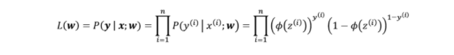
Figure 2: Maximum likelihood curve for logistic regression

For mathematical simplicity, the method of obtaining the negative log of the likelihood method (as described above) and reducing the function is used to maximize the likelihood function. As a result, log loss is another name for cross-entropy loss. Because it is simple to compute the derivative of the resulting summation method after taking the log, it makes it simple to minimize the negative log-likelihood function. Here is a picture of the probability function's log from earlier.

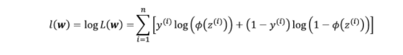
Figure 3: Logistic Regression's log-likelihood function

The -ve (negative) of the log-likelihood method as illustrated in fig. 3 is chosen in order to perform gradient descent to the log-likelihood function mentioned before. As a result, for y = 0 and y = 1, the cost method matches that shown in figure 1.

Plotting the log-loss function or cross-entropy loss function versus the probability value/hypothesis outcome will look like the following:

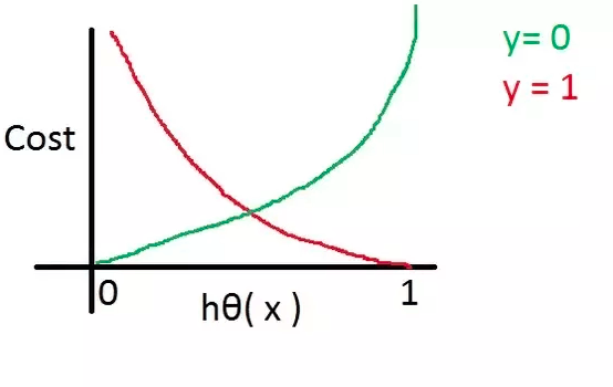
Fig 4. Learning the log loss function or cross-entropy for Logistic Regression

Let's examine the log loss function in the context of the illustration above:

• If the assumption value is 1, the cost or loss function result for the actual label value of 1 (red line) will be close to zero. But the price will be quite high if the assumption value is 0 (near to infinite).
• If the assumption value is 1, the output of the loss or cost function for the actual label value of 0 (green line) will be close to infinity. The cost will be significantly lower, though, if the assumption value is 0 (near zero).

Based on the foregoing, the logistic regression model or models that use the softmax method as an activation function, such as a neural network, can learn their parameters using the gradient descent algorithm.

Explanation of Cross-entropy Loss Using a Python Example

With the help of Python code examples, you will study cross-entropy loss in this part. This is the method that we must translate into a Python function.

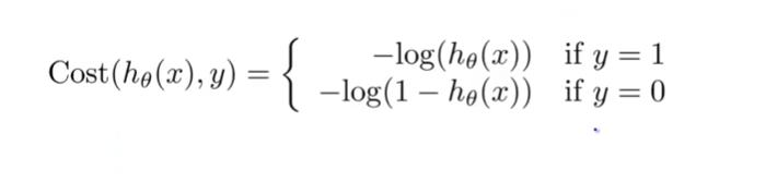
Figure 5. Cross-Entropy Loss Function.

According to the aforementioned function, we require two functions: one that represents the equation in Fig. 5 as a cost method (cross-entropy function), and the other that generates the probability. The sigmoid function used in this section is the hypothesis function. Below is provided the Python code for each of these two functions. Pay close attention to the cross-entropy loss method (cross-entropy loss) and the sigmoid function (hypothesis).

import numpy as np
import matplotlib.pyplot as plt


'''
Hypothesis method - Sigmoid method
'''
def sigmoid(a):
    return 1.0 / (1.0 + np.exp(-a))


'''
The predicted value or probability value calculated as a result of the hypothesis or sigmoid function is represented by y_Hat.


y stands for the real label.
'''
def cross_entropy_loss(y_Hat, y):
    if y == 1:
      return -np.log(y_Hat)
    else:
      return -np.log(1 - y_Hat)

Once we have two functions, let's generate a sample value of a (weighted total as in logistic regression) and a cross-entropy loss function plot that contrasts the output of the cost function and the output of the hypothesis function (probability value).

# Determine sample values for a


a = np.arange(-10, 10, 0.1)


# Determine the probability value/ hypothesis value 


h_a = sigmoid(a)


# Cost function value when y = 1
# -log(h(x))


cost__1 = cross_entropy_loss(h_a, 1)


# Value of cost function when y = 0
# -log(1 – h(x))
#
cost_0 = cross_entropy_loss(h_a, 0)


# Plot the loss in cross-entropy


figr, a_x = plot.subplots(figsize=(8,6))
plot.plot(h_a, cost__1, label='J(w) if y=1')
plot.plot(h_a, cost_0, label='J(w) if y=0')
plot.xlabel('$\phi$(a)')
plot.ylabel('J(w)')
plot.legend(loc='best')
plot.tight_layout()
plot.show()

The cross-entropy loss or log loss plot would seem as follows:

Cost function vs probability (Hypothesis Function Output)

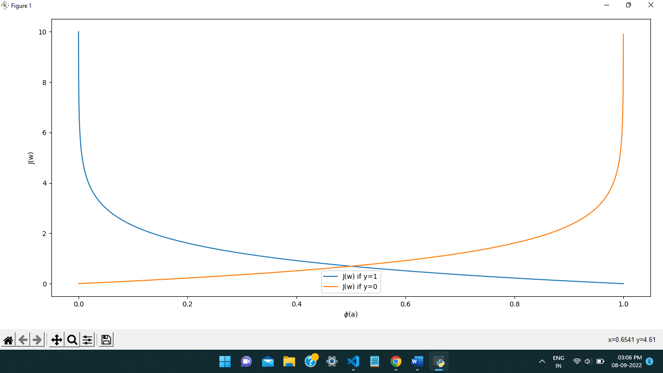
Figure 6: Cross-Entropy Loss Function Plot.

In the example above, take note of the following:

For y = 1, the loss function out, J(W), is near zero if the anticipated probability is nearone; otherwise, it is near to infinity.

The loss function out, J(W), is near zero for y = 0 if the anticipated probability is nearzero, else it is near to infinity.

Conclusions

The summary of your education regarding the cross-entropy loss function is as follows:

In order to estimate the parameters for models with softmax output or logistic regression models, the cross-entropy loss function is utilized as an optimization function.

When discussing logistic regression, the log loss function is another name for the cross-entropy loss function. This is due to the log-likelihood function's negative being minimized.

When the anticipated probability is drastically different from the actual class label, the cross-entropy loss is large (0 or 1).

When the projected probability is more or less like the actual class label, the cross-entropy loss is reduced (0 or 1).

The model parameters can be calculated using a cross-entropy loss function and a gradient descent approach.