In this article, we'll walk through a tutorial for utilising the Python Sklearn (formerly known as Scikit Learn) package to implement logistic regression. To assist you in remembering the concept, we'll give you a quick explanation of logistic regression. After that, we'll create an entire project using a dataset to demonstrate Sklean logistic regression using the Logistic Regression() method.

Now let’s start with the basic introduction of Logistic Regression in Python.

Introduction of Logistic Regression in Python

A statistical method for classifying objects is logistic regression.

For a better understanding of Logistic regression in Python, let’s move on to its classification.

We need to understand what categorization entails to comprehend logistic regression. To further grasp this, let's look at the samples below:

The tumor is categorized as benign or malignant by a doctor.
A bank transaction could be legitimate or fraudulent.

Logistic regression is one component of machine learning that addresses this type of binary classification challenge. Other machine learning methods have been created and are currently being used to address various other issues.

Let’s understand the Logistic Regression in Python by taking an example given below:

Example

# importing dataset and logistic regression model libraries
# iris dataset imported
from sklearn.datasets import load_iris
# logistic regression model imported
from sklearn.linear_model import LogisticRegression


# loading data set into x and y variables
X, y = load_iris(return_X_y=True)


# creating the object of LogisticRegression
log_model = LogisticRegression(random_state=0)


# training the model
log_model.fit(X, y)


# testing the model
test_result = log_model.predict(X[45: 55, :])
print("output of the test input is:", test_result)


# checking the precision of the model
precision = log_model.score(X, y)
print("The precision of the model:", precision)

Output

output of the test input is: [0 0 0 0 0 1 1 1 1 1]
The precision of the model: 0.9733333333333334

The example above uses the iris data set for our training and testing of the logistic regression model. First, we imported all the needed libraries. We created 2 variables X and y, and we trained our model.

We check the precision of the model by using the score() method. And we have the given result.

There are other classification issues where more than two classes may be possible. We can be requested to separate different fruits from each other after being given a basket full of fruits. The multivariate categorisation is needed.

Let’s know what the syntax of Logistic Regression is.

Syntax of Logistic Regression

Syntax of logistic regression is given below

Class sklearn.linear_model.LogisticRegression(penalty='l2', *, dual=False, tol=0.0001, C=1.0, fit_intercept=True, intercept_scaling=1, class_weight=None, random_state=None, solver='lbfgs', max_iter=100, multi_class='auto', verbose=0, warm_start=False, n_jobs=None, l1_ratio=None)

Here we can see that Logistic regression has a lot of parameters. Let’s understand these parameters one by one.

Parameters

Penalty: penalty may have values: “none,” “l1, “ “l2”, and “elasticnet. No penalty will be applied when the penalty parameter is set to zero. When the penalty parameter is set to l1, the l1 penalty is applied. When the penalty parameter has elasticnet, both l1 and l2 penalties are applied.
Dual: dual parameter can take the value true or false. If the dual set to the value is true, then the model works on the dual formulation. It is implemented only for the l2 penalty. The default value is false. The model works on the primal formulation.
Tol: This instructs Scikit to give up looking for a minimum (or maximum) if a certain level of tolerance is reached. The default value of tol is “1e-4.”
C: Negative float; the inverse of regularisation strength. A higher regularisation is indicated by smaller values, just like in support vector machines.
Float, default is 1.0.
fit_intercept: specifies whether the decision function should include a constant (also known as a bias or intercept).
Bool, the default is True.
intercept_scaling: Useful only if self.fit intercept is set to True, and the solver 'liblinear' is employed. A "synthetic" feature with a constant value equal to intercept scaling is added to the instance vector, making x become [x, self.intercept scaling]. Synthetic feature weight multiplied by intercept scaling yields the intercept.

Please note that, like all other features, the synthetic feature weight is subject to l1/l2 regularisation. It is necessary to boost intercept scaling to decrease the impact of regularisation on synthetic feature weight (and hence on the intercept).
Float, default is 1.
class_weight: Weights with the format "class label: weight" are linked to certain classes. All classes are expected to have weight one if it is not provided.
As n samples / (n classes * np.bincount(y)), the "balanced" mode automatically adjusts weights inversely proportional to class frequencies in the input data.

If sample weight is supplied, it should be noted that these weights will be multiplied by sample weight and passed via the fit function.
random_state: Used to shuffle the data when solver == "sag," "saga," or "liblinear." For more information, consult the glossary.
Int, RandomState instance, default is None.
Solver: The optimisation problem's algorithm. "lbfgs" is the default. You may want to take into account the following factors while selecting a solver:
- "Liblinear" is a decent option for small datasets, but "sag" and "saga" are quicker for large datasets;
- Only "newton-cg," "sag," "saga," and "lbfgs" handle multinomial loss in multiclass situations;
- The term "liblinear" is only applicable to one-versus-rest schemes.
  
  {‘newton-cg’, ‘lbfgs’, ‘liblinear’, ‘sag’, ‘saga’}, default=’lbfgs’
max_iter: The most iterations necessary for the solvers to converge. Int, default is 100.
multi_class: For each label, a binary problem fits if the option selected is "ovr." If the data is binary or solver='liblinear,' 'auto' chooses 'ovr'; else, chooses'multinomial'. Even when the data is binary, the multinomial loss fit throughout the full probability distribution is the loss that is minimised for "multinomial." When solver='liblinear,' multinomial is not available.

{‘auto’, ‘ovr’, ‘multinomial’}, default is ’auto’.
Verbose: Set verbose to any positive number for verbosity for the liblinear and lbfgs solvers.
Int, default is 0.
warm_start: When set to True, the solution from the prior call is used as initialisation; otherwise, the prior solution is simply erased. For the liblinear solver useless.
Bool, the default is False.
n_jobs: if multi class='ovr', the number of CPU cores utilised while parallelising over classes. Whether or not 'multi_class' is supplied, this argument is ignored when the solver is set to 'liblinear'. Except in a joblib.parallel backend environment, none means 1. Using all processors equals -1.
Int, default is None.
L1_ratio: Elastic-Net mixing parameter, where l1 ratio ranges from 0 to 1. Applied only when penalty='elasticnet'. While using penalty='l2' while setting l1 ratio=0, using penalty='l1' when setting l1 ratio=1 is comparable. The penalty is a combination of L1 and L2 for an l1 ratio of 0 to 1.
Float, default is None.

Here we can see that Logistic regression has a lot of attributes. Let’s understand these attributes one by one.

Attributes

1. classes_: a list of the classifier's recognised class labels. It is an attribute in this.
ndarray of shape (n_classes, )

2. coef_: coefficient of the decision function's characteristics.

When the supplied problem is binary, coef_ has the shape (1, n features). Coef_ corresponds to outcome 1 (True) when multi class='multinomial,' whereas -coef_ corresponds to outcome 0. (False).

ndarray of shape (1, n_features) or (n_classes, n_features)

3. intercept_: added intercept (also known as bias) to the decision function.

The intercept is 0 if the fit intercept is set to False. In cases when the presented problem is binary, intercept_ has the shape (1,). For example, when multi class='multinomial,' intercept_ corresponds to result from 1 (True), and -intercept_ to outcome 0. (False).

ndarray of shape (1,) or (n_classes,)

4. n_features_in_: number of features noticed when fitting.

It's Updated in version 0.24.

The data type of this attribute is Int.

5. feature_names_in_: characteristics identified by names during a fit. X is only defined when all of its feature names are strings.

It's Updated in version 1.0.

ndarray of shape (n_features_in_,)

6. n_iter_: Number of actual iterations for each class. Only the maximum number of iterations across all classes is provided for the liblinear solver. It only returns 1 element if the input is binary or multinomial.

Updated in version 0.20: n iter_ will now report at most max iter in SciPy versions greater than 1.0.0, where the number of lbfgs iterations may exceed max iter.

ndarray of shape (n_classes,) or (1, )

Creating Logistic Regression Model

Step by step, let’s understand how to create a LinearRegression model using sklearn in python.

1st step

Let’s start creating LogisticRegression Model by the following 1 step.

1st we must import all required libraries such as numpy, pandas, and seaborn.

Basically, in this step, we are going to load the libraries.

# importing required libraries
# importing numpy and pandas for data structure
import numpy as np
import pandas as pd
# importing sklearn libraries required for training the model
from sklearn.model_selection import train_test_split
from sklearn.preprocessing import StandardScaler
from sklearn.pipeline import Pipeline
from sklearn.metrics import roc_curve, roc_auc_score, classification_report, accuracy_score, confusion_matrix 
# importing seaborn and matplotlib.pyplot for visualisation
import seaborn as sns
import matplotlib.pyplot as plt
# iris dataset imported for training and testing the model
from sklearn.datasets import load_iris
# logistic regression model imported
from sklearn.linear_model import LogisticRegression

Scikit-learn uses the SciPy stack's libraries in the order described below for data analysis.

Numpy - This library or module has Advanced linear algebraic and array operations.
SciPy - Has modules for linear algebra, optimisation, and other crucial data science operations.
IPython - Increasing interactivity on consoles.
Matplotlib - Data visualisation and graphing in two or three dimensions using Matplotlib.
SymPy - used for Computer algebra and symbolic computation.
Pandas - A data analysis and manipulation tool primarily using dataframes and tables.

2nd step

After performing 1 st step, Let’s move on to the second step.

For the logistic regression model, we use the built-in datasets stored in sklearn.dataset library. As we can see below, the dataset is enormous; therefore, for this tutorial's purposes, we'll be concentrating on two key columns.

Basically, in this step, we are going to load the dataset.

Let’s understand this by taking an example given below:

Example

# importing required libraries
# importing numpy and pandas for data structure
import numpy as np
import pandas as pd
# importing sklearn libraries required for training the model
from sklearn.model_selection import train_test_split
from sklearn.preprocessing import StandardScaler
from sklearn.pipeline import Pipeline
from sklearn.metrics import roc_curve, roc_auc_score, classification_report, accuracy_score, confusion_matrix
# importing seaborn and matplotlib.pyplot for visualisation
import seaborn as sns
import matplotlib.pyplot as plt
# iris dataset imported for training and testing the model
from sklearn.datasets import load_iris
# logistic regression model imported
from sklearn.linear_model import LogisticRegression


# loading data set into x and y variables
X, y = load_iris(return_X_y=True)
x_df = pd.DataFrame(data=X, columns=load_iris().feature_names)
print(f'''table
{x_df.head()}


description
{x_df.describe()}
''')

Output:

table
   	sepal length (cm)  	sepal width (cm)  	petal length (cm)  	petal width (cm)
0                5.1               		3.5                		1.4               		0.2
1                4.9               		3.0                		1.4               		0.2
2                4.7               		3.2                		1.3               0.2
3                4.6               		3.1                		1.5               0.2
4                5.0               		3.6                		1.4               0.2


description
       	sepal length (cm)  	sepal width (cm)  	petal length (cm)  	petal width (cm)
count	  50.000000        	150.000000         	150.000000        	150.000000
mean     5.843333          	3.057333           	3.758000          	1.199333
std         0.828066          	0.435866           	1.765298          	0.762238
min       4.300000          	2.000000           	1.000000          	0.100000
25%      5.100000          	2.800000           	1.600000          	0.300000
50%      5.800000          	3.000000           	4.350000          	1.300000
75%      6.400000          	3.300000           	5.100000          	1.800000
max      7.900000          	4.400000           	6.900000          	2.500000

3rd step

After performing 2 nd step, Let’s move on to the third step.

The first step will separate the dependent variable from the independent variables in data frame Y.

The train_test_split() function was then used to divide the dataset into training and testing sets.

Basically, in this step, we will split the dataset into the Training and Test sets.

Let’s understand this by taking an example given below:

Example

# importing required libraries
# importing numpy and pandas for data structure
import numpy as np
import pandas as pd
# importing sklearn libraries required for training the model
from sklearn.model_selection import train_test_split
from sklearn.preprocessing import StandardScaler
from sklearn.pipeline import Pipeline
from sklearn.metrics import roc_curve, roc_auc_score, classification_report, accuracy_score, confusion_matrix
# importing seaborn and matplotlib.pyplot for visualisation
import seaborn as sns
import matplotlib.pyplot as plt
# iris dataset imported for training and testing the model
from sklearn.datasets import load_iris
# logistic regression model imported
from sklearn.linear_model import LogisticRegression


# loading data set into x and y variables
X, y = load_iris(return_X_y=True)




# splitting our data into test data and training data
X_train, X_test, y_train, y_test = train_test_split(X, y, test_size=.25, random_state=0)

4th step

After performing 3 rd step, Let’s move on to the fourth step.

StandardScaler carries out the task of standardisation. Different scales of variable values can be found in our dataset. While creating a machine learning model, several columns with multiple scales are standardised to have a similar scale.

Let’s understand this by taking an example given below:

Example

# importing required libraries
# importing numpy and pandas for data structure
import numpy as np
import pandas as pd
# importing sklearn libraries required for training the model
from sklearn.model_selection import train_test_split
from sklearn.preprocessing import StandardScaler
from sklearn.pipeline import Pipeline
from sklearn.metrics import roc_curve, roc_auc_score, classification_report, accuracy_score, confusion_matrix
# importing seaborn and matplotlib.pyplot for visualisation
import seaborn as sns
import matplotlib.pyplot as plt
# iris dataset imported for training and testing the model
from sklearn.datasets import load_iris
# logistic regression model imported
from sklearn.linear_model import LogisticRegression


# loading data set into x and y variables
X, y = load_iris(return_X_y=True)




# splitting our data into test data and training data
X_train, X_test, y_train, y_test = train_test_split(X, y, test_size=.25, random_state=0)


# scaling the x data set
sc = StandardScaler()
X_train = sc.fit_transform(X_train)
X_test = sc.transform(X_test)

5th step

After completing the 4th step, Let’s move on to the 5th step.

Here we are creating the logistic model we need to train using our train data. To create the logistic, we must create an instance of LogisticRegression(). Then we will train it using the fit() method. Here we are not passing any argument in the LogisticRegression(), so it will take the default parameter values.

Let’s understand this by taking an example given below:

Example

# importing required libraries
# importing numpy and pandas for data structure
import numpy as np
import pandas as pd
# importing sklearn libraries required for training the model
from sklearn.model_selection import train_test_split
from sklearn.preprocessing import StandardScaler
from sklearn.pipeline import Pipeline
from sklearn.metrics import roc_curve, roc_auc_score, classification_report, accuracy_score, confusion_matrix
# importing seaborn and matplotlib.pyplot for visualisation
import seaborn as sns
import matplotlib.pyplot as plt
# iris dataset imported for training and testing the model
from sklearn.datasets import load_iris
# logistic regression model imported
from sklearn.linear_model import LogisticRegression


# loading data set into x and y variables
X, y = load_iris(return_X_y=True)




# splitting our data into test data and training data
X_train, X_test, y_train, y_test = train_test_split(X, y, test_size=.25, random_state=0)


# scaling the x data set
sc = StandardScaler()
X_train = sc.fit_transform(X_train)
X_test = sc.transform(X_test)


# creating the model and training the model
logistic_model = LogisticRegression()
# training the model with the train data, i.e. X_train, y_train
logistic_model.fit(X_train, y_train)

6th step

After completing the 5th step, Let’s move on to the 6th step.

In this step, we will predict the result of our test data and match it with the original data. We will check the accuracy of our model. And we will try to find what per cent of the data matches all results.

Let’s understand this by taking an example given below:

Example

# importing required libraries
# importing numpy and pandas for data structure
import numpy as np
import pandas as pd
# importing sklearn libraries required for training the model
from sklearn.model_selection import train_test_split
from sklearn.preprocessing import StandardScaler
from sklearn.pipeline import Pipeline
from sklearn.metrics import roc_curve, roc_auc_score, classification_report, accuracy_score, confusion_matrix
# importing seaborn and matplotlib.pyplot for visualisation
import seaborn as sns
import matplotlib.pyplot as plt
# iris dataset imported for training and testing the model
from sklearn.datasets import load_iris
# logistic regression model imported
from sklearn.linear_model import LogisticRegression


# loading data set into x and y variables
X, y = load_iris( return_X_y=True )




# splitting our data into test data and training data
X_train, X_test, y_train, y_test = train_test_split(X, y, test_size=.25, random_state=0)


# scaling the x data set
sc = StandardScaler()
X_train = sc.fit_transform( X_train )
X_test = sc.transform( X_test )


# creating model
logistic_model = LogisticRegression()
logistic_model.fit( X_train, y_train )


# precision of the model for train dataset
train_precision = logistic_model.score( X_train, y_train )


# precision of the model for test dataset
test_precision = logistic_model.score( X_test, y_test )


# prediction by the model
y_pred = logistic_model.predict( X_test )


probability = logistic_model.predict_proba( X_test )
percent_setosa = list( map( lambda x: round(x[0]*100, 2), probability ))
percent_versicolor = list( map( lambda x: round(x[1]*100, 2), probability ))
percent_virginica = list( map( lambda x: round(x[2]*100, 2), probability ))
pred_table = pd.DataFrame(data={
    "original data": list( map( lambda i: load_iris().target_names[i], y_test )),
    "prediction": list( map( lambda i: load_iris().target_names[i], y_pred )),
    "setosa(%)": percent_setosa,
    "versicolor(%)": percent_versicolor,
    "virginica(%)": percent_virginica
})


print(f'''precision of the model for train dataset: {train_precision}
precision of the model for test dataset: {test_precision}


prediction table
{pred_table.head( 10 )}
''')

Output

precision of the model for train dataset: 0.9732142857142857
precision of the model for test dataset: 0.9736842105263158


prediction table
  	original data  	prediction  	setosa(%)  	versicolor(%)  	virginica(%)
0     	virginica   	virginica       	0.01           	3.10         		96.88
1    	versicolor  	versicolor      	0.61          	95.18          		4.21
2        	setosa      	setosa      	99.58           	0.42          		0.00
3     	virginica   	virginica       	0.00           	8.17         		91.83
4        	setosa      	setosa      	97.61           	2.39          		0.00
5     	virginica   	virginica       	0.00           	1.00         		98.99
6       	setosa      	setosa      	98.34           	1.66          		0.00
7    	versicolor  	versicolor      	0.72          	71.49         		27.79
8    	versicolor  	versicolor      	0.24          	72.88         		26.88
9    	versicolor  	versicolor      	2.31          	89.39          		8.29

7th step

After completing the 6th step, Let’s move on to the 7th step.

For more clarity, let's utilise the classification_report() function to determine the model's precision and recall for the test dataset. Here f1-score shows how many items from the test dataset has identified in the form of a per cent. It will show all states like precision for the value 1, 2, and 3, average, weight average, etc.

Let’s understand this by taking an example given below:

Example

# importing required libraries
# importing numpy and pandas for data structure
import numpy as np
import pandas as pd
# importing sklearn libraries required for training the model
from sklearn.model_selection import train_test_split
from sklearn.preprocessing import StandardScaler
from sklearn.pipeline import Pipeline
from sklearn.metrics import roc_curve, roc_auc_score, classification_report, accuracy_score, confusion_matrix
# importing seaborn and matplotlib.pyplot for visualisation
import seaborn as sns
import matplotlib.pyplot as plt
# iris dataset imported for training and testing the model
from sklearn.datasets import load_iris
# logistic regression model imported
from sklearn.linear_model import LogisticRegression


# loading data set into x and y variables
X, y = load_iris( return_X_y=True )




# splitting our data into test data and training data
X_train, X_test, y_train, y_test = train_test_split(X, y, test_size=.25, random_state=0)


# scaling the x data set
sc = StandardScaler()
X_train = sc.fit_transform( X_train )
X_test = sc.transform( X_test )


# creating model
logistic_model = LogisticRegression()
logistic_model.fit( X_train, y_train )


# precision of the model for train dataset
train_precision = logistic_model.score( X_train, y_train )


# precision of the model for test dataset
test_precision = logistic_model.score( X_test, y_test )


# prediction by the model
y_pred = logistic_model.predict( X_test )


probability = logistic_model.predict_proba( X_test )
percent_setosa = list( map( lambda x: round(x[0]*100, 2), probability ))
percent_versicolor = list (map( lambda x: round(x[1]*100, 2), probability ))
percent_virginica = list( map( lambda x: round(x[2]*100, 2), probability ))
pred_table = pd.DataFrame(data={
    "original data": list( map( lambda i: load_iris().target_names[i], y_test )),
    "prediction": list( map( lambda i: load_iris().target_names[i], y_pred )),
    "setosa(%)": percent_setosa,
    "versicolor(%)": percent_versicolor,
    "virginica(%)": percent_virginica
})


# getting the report of classification in detail
report = classification_report( y_test, y_pred )
print(f'''detailed report of our model for the test dataset
{report}''')

Output:

detailed report of our model for the test dataset
              	    precision 	recall 	f1-score   support


           0       	    1.00      	1.00    	1.00    		13
           1       	    1.00      	0.94    	0.97        	16
           2       	    0.90      	1.00    	0.95         	9


accuracy                           		0.97        	38
macro avg         0.97      	0.98    0.97        	38
weighted avg    0.98      	0.97    0.97        	38

8th step

After completing the 7th step, Let’s move on to the 8th step.

In this step, we will make a confusion matrix. The confusion matrix is a matrix that shows the performance classification algorithm that our model is using. In sklearn, we have a built-in module to build a confusion matrix named confusion_matrix(y_test, y_pred).

Let’s understand this by taking an example given below:

Example

# importing required libraries
# importing numpy and pandas for data structure
import numpy as np
import pandas as pd
# importing sklearn libraries required for training the model
from sklearn.model_selection import train_test_split
from sklearn.preprocessing import StandardScaler
from sklearn.pipeline import Pipeline
from sklearn.metrics import roc_curve, roc_auc_score, classification_report, accuracy_score, confusion_matrix
# importing seaborn and matplotlib.pyplot for visualisation
import seaborn as sns
import matplotlib.pyplot as plt
# iris dataset imported for training and testing the model
from sklearn.datasets import load_iris
# logistic regression model imported
from sklearn.linear_model import LogisticRegression


# loading data set into x and y variables
X, y = load_iris( return_X_y=True )




# splitting our data into test data and training data
X_train, X_test, y_train, y_test = train_test_split( X, y, test_size=.25, random_state=0)


# scaling the x data set
sc = StandardScaler()
X_train = sc.fit_transform( X_train )
X_test = sc.transform( X_test )


# creating model
logistic_model = LogisticRegression()
logistic_model.fit( X_train, y_train )


# precision of the model for train dataset
train_precision = logistic_model.score( X_train, y_train )


# precision of the model for test dataset
test_precision = logistic_model.score( X_test, y_test )


# prediction by the model
y_pred = logistic_model.predict( X_test )


probability = logistic_model.predict_proba( X_test )
percent_setosa = list( map( lambda x: round(x[0]*100, 2), probability ))
percent_versicolor = list( map( lambda x: round(x[1]*100, 2), probability ))
percent_virginica = list( map( lambda x: round(x[2]*100, 2), probability ))
pred_table = pd.DataFrame(data={
    "original data": list( map( lambda i: load_iris().target_names[i], y_test )),
    "prediction": list( map( lambda i: load_iris().target_names[i], y_pred )),
    "setosa(%)": percent_setosa,
    "versicolor(%)": percent_versicolor,
    "virginica(%)": percent_virginica
})


# getting the report of classification in detail
report = classification_report( y_test, y_pred )
# print(f'''detailed report of our model for the test dataset
#{report}''')


# creating confusion matrix by using confusion_matrix() function
c_mat = confusion_matrix( y_test, y_pred )
print(f'''Confusion matrix:
{c_mat}
''')

Output

Confusion matrix:
[[13  0  0]
 [ 0 15  1]
 [ 0  0  9]]

9th step

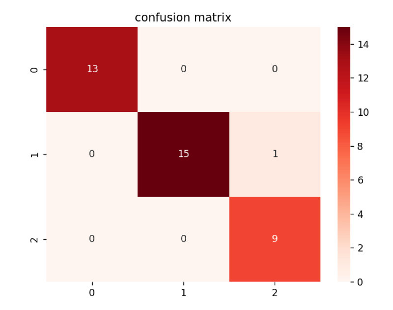
After completing the 8th step, Let’s move on to the 9th step.

In sklearn, we have a built-in module to build a confusion matrix named confusion_matrix( y_test, y_pred ). In this step, we will visualise the confusion matrix we created in the previous step. Now we will use pyplot and seaborn to visualise the confusion matrix. We will use the sns.heatmap() function to visualise the confusion matrix.

Let’s understand this by taking an example given below:

Example

# importing required libraries
# importing numpy and pandas for data structure
import numpy as np
import pandas as pd
# importing sklearn libraries required for training the model
from sklearn.model_selection import train_test_split
from sklearn.preprocessing import StandardScaler
from sklearn.pipeline import Pipeline
from sklearn.metrics import roc_curve, roc_auc_score, classification_report, accuracy_score, confusion_matrix
# importing seaborn and matplotlib.pyplot for visualisation
import seaborn as sns
import matplotlib.pyplot as plt
# iris dataset imported for training and testing the model
from sklearn.datasets import load_iris
# logistic regression model imported
from sklearn.linear_model import LogisticRegression


# loading data set into x and y variables
X, y = load_iris( return_X_y=True )




# splitting our data into test data and training data
X_train, X_test, y_train, y_test = train_test_split( X, y, test_size=.25, random_state=0)


# scaling the x data set
sc = StandardScaler()
X_train = sc.fit_transform( X_train )
X_test = sc.transform( X_test )


# creating model
logistic_model = LogisticRegression()
logistic_model.fit( X_train, y_train )


# precision of the model for train dataset
train_precision = logistic_model.score( X_train, y_train )


# precision of the model for test dataset
test_precision = logistic_model.score( X_test, y_test )


# prediction by the model
y_pred = logistic_model.predict( X_test )


probability = logistic_model.predict_proba( X_test )
percent_setosa = list( map( lambda x: round(x[0]*100, 2), probability ))
percent_versicolor = list( map( lambda x: round(x[1]*100, 2), probability ))
percent_virginica = list( map( lambda x: round(x[2]*100, 2), probability ))
pred_table = pd.DataFrame( data={
    "original data": list( map( lambda i: load_iris().target_names[i], y_test )),
    "prediction": list( map( lambda i: load_iris().target_names[i], y_pred )),
    "setosa(%)": percent_setosa,
    "versicolor(%)": percent_versicolor,
    "virginica(%)": percent_virginica
})


# getting the report of classification in detail
report = classification_report(y_test, y_pred)


# creating confusion matrix by using confusion_matrix() function
c_mat = confusion_matrix(y_test, y_pred)


sns.heatmap(c_mat, annot=True, cmap="Reds")
plt.title("confusion matrix")
plt.show()

Output

Python Logistic Regression with Sklearn & Scikit

Conclusion

We hope you enjoyed our article and know how to use Sklearn (Scikit Learn) to create logistic regression in Python(Implementation of logistic regression using the Scikit-Learn framework on the IRIS Dataset). We gave you a step-by-step example of how to use a dataset and the SKlearn LogisticRegression() function to build a logistic regression model for a prediction task. The tutorial also demonstrates that we shouldn't rely on accuracy scores to assess how well-imbalanced datasets perform.

Python Tutorial

Python Conditional Statements

Python Loops

Python Arrays

Python Strings

Python Built-in Data Structure

Python Functions

Python File Handling

Python Exception Handling

Python OOPs Concept

Python Iterators

Python Generators

Python Decorators

Python Functions and Methods

Python Modules

Python MySQL

Python MongoDB

Python SQLite

Python Data Structure Implementation

Python Advance Topics

Python 2

Python 3

How to

Sorting

Programs

Questions

Differences

Python Kivy

Python Tkinter

Python PyQt5

Python PyGal

Misc

Python Logistic Regression with Sklearn & Scikit

Introduction of Logistic Regression in Python

Syntax of Logistic Regression

Parameters

Attributes

Creating Logistic Regression Model

Conclusion