XGBoost for Regression in Python

Regression problem results real values. Decision Trees and Linear Regression are regularly used regression algorithms and use some metrics involved in regression like mean squared error and root mean squared error. These metrics plays major role in XGBoost models.

• Mean squared error: It is a sum of original and assumed differences, but it unavailability in mathematically, that’s it not used commonly, as compared to other metrics.
• Root mean squared error: This metric is square root of MSE.

XGBoost are used to build the execution of regression models. Base learners and objective function will conclude the validity of a statement. The objective function contains loss function. This function will talk about the difference between assumed values and original values that is it calculates the model results from the real values. Regression problems most common loss function of XGBoost are reg: linear and for binary is reg: logistics. One approach to group learning is XGBoost. When all the predictions are merged, bad predictions cancel out and better ones add up to generate final good predictions, which is what XGBoost anticipates to have base learners who are uniformly bad at the rest.

Python Programs

Example 1:

// python program
// importing packages
importnumpy as a
importpandas as c
importxgboost as g
fromsklearn.model_selection importtrain_test_split
fromsklearn.metrics importmean_squared_error as MSE
 
// Loading the data
dataset =a.read_csv("boston_house.csv")
J, i =dataset.iloc[:, :-1], dataset.iloc[:, -1]
 
// Splitting the data
train_J, test_J, train_i, test_i =train_test_split(J, i,
                      test_size =0.3, random_state =123)
 
// Installing the data
gb_r =g.XGBRegressor(objective ='reg:linear',
                  n_estimators =10, seed =123)
 
// Fitting the model
gb_r.fit(train_J, train_i)
 
// Predict the model
pred =gb_r.predict(test_J)
 
//root mean squared error Computation
rmse =a.sqrt(MSE(test_i, pred))
print("RMSE: %f" %(rmse))

Output:

129043.2314

Example 2:

// python program for linear base learner
// importing the packages
importnumpy as a
importpandas as c
importxgboost as g
fromsklearn.model_selection importtrain_test_split
fromsklearn.metrics importmean_squared_error as MSE
 
// Loading the data
dataset =a.read_csv("boston_house.csv")
J, i =dataset.iloc[:, :-1], dataset.iloc[:, -1]
 
// Splitting the data
train_J, test_J, train_i, test_i =train_test_split(J, i,
                      test_size =0.3, random_state =123)
 
// Train and test set are converted to DMatrix objects.
train_dmatrix =g.DMatrix(data =train_J, label =train_i)
test_dmatrix =g.DMatrix(data =test_J, label =test_i)
 
// Parameter dictionary specifying base learner
param ={"booster":"gblinear", "objective":"reg:linear"}
 
gb_r =g.train(params =param, dtrain =train_dmatrix, num_boost_round =10)
pred =gb_r.predict(test_dmatrix)
 
// Root mean squared error Computation
rmse =a.sqrt(MSE(test_i, pred))
print("RMSE: %f" %(rmse))

Output:

12326.24465

The dataset needs to be transferred into DMatrix. It is an advance data structure that generates of XGBoost made.Performance and effectiveness will deliver the whole package. The complexity of the model depends on the analyses of the loss function, and as the model complexity increases, regularisation can be used to penalise the model. In order to avoid overfitting, it penalises more complicated models using both LASSO (L1) and Ridge (L2) regularisation. Finding precise and straightforward models is the result.

Regularization parameters are three types:

1. Lambda
2. Gamma
3. Alpha

• Gamma: It is a minimum depletion of loss allow to occur a split. If we increase the gamma, splits will reduce.
• Alpha: L1 regularization has large value on leaf weights, so it causes base learner to go to 0 in leaf weights.
• Lambda: L2 regularization has low and easy than L1 and it causes smoothly and easily to reduce on leaf weights.

Regression of XGBoost tree:

Step 1: Calculate the same scores for increasing the tree.

Same Score = (Sum of residuals)^2 / Number of residuals + lambda

Step 2: Calculate the gain to know how to divide the data.

Gain = Left tree (same score) + Right (same score) - Root (same score)

Step 3: Calculate the difference between gamma and gain

Gain -gamma

If the result is a positive number go to next step if not positive number, then prune.

Step 4: Calculate result of another leaves:

result value = Sum of residuals / Number of residuals + lambda.

When lambda is greater than 0, the similarity scores are reduced, which leads to more pruning and smaller leaf output values. Let's examine a portion of mathematics involved in determining the appropriate output value to minimise the loss function. XGBoost starts with an initial prediction, often 0.5, for classification and regression.

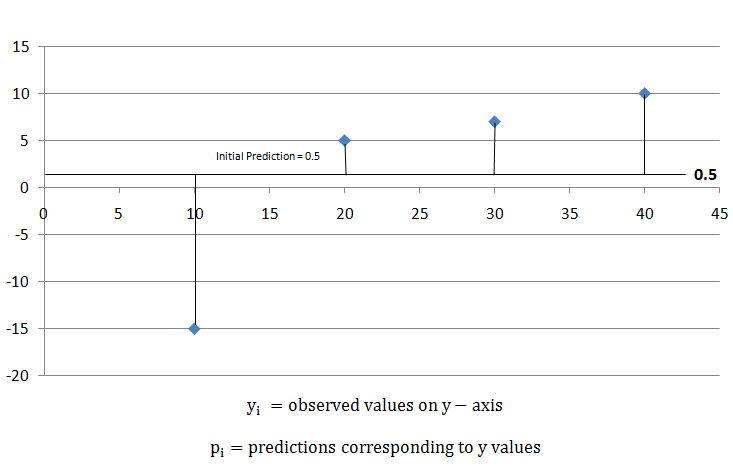
Calculate the loss function

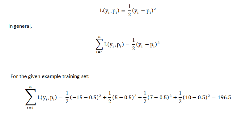
It came to be 196.5 in the scenario of the example given. Later, we can apply this loss function, compare the outcomes, and determine whether or not estimates are becoming better. By reducing the formula given, XGBoost builds trees using those loss functions:

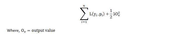
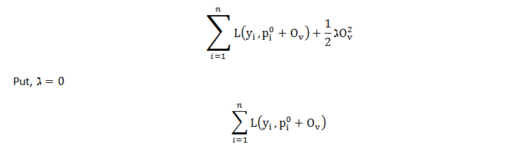
The loss function and regularisation term make up the first and second parts of the equation, and the aim is to minimise the overall system. We write the equation as follows to maximise the output value for the first tree. For simpler calculations, we replace p(i) with the initial predictions and output value.

The loss function for the initially assumed was already calculated and caught to be 196.5. Thus, loss function equals 196.5 for result value of 0. Similar to the last example, if we plot the point for result value = -1, loss function = 203.5, for result value = +1, loss function = 193.5, and so on for other result values, we get a design that looks a parabola. The equation's plot as a method of the result values.

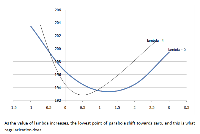
The best output value can be found near the parabola's bottom, where the derivation is zero, if lambda = 0. XGBoost uses the Second-Order Taylor Approximation for both regression and classification. An approximate representation of the loss function with outcome values is given below:

XGBoost selects Taylor Approximation for both classification and regression. An approximate representation of the loss function with outcome values. The first derivative in this case is connected to Gradient Descent, so XGBoost represents it with the letter "g," and the second derivative is related to Hessian, so XGBoost represents it with the letter "h."

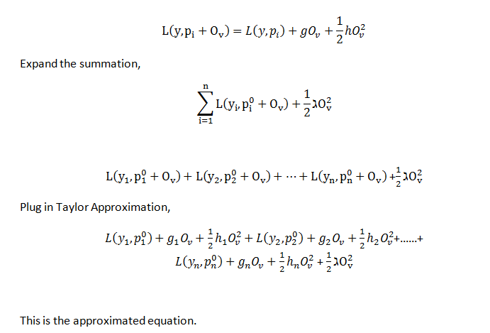
Removing the values which doesn’t contain result value, minimizing the left-over function:

• Take result value as per derivation
• Set derivative = 0
• g (i) = negative residual
• h (i) = total no.of residual

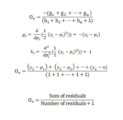
This is the result value as per formula for XGBoost in regression.