Sklearn linear Model in Python

The most effective and reliable Python machine learning library is Sklearn. Through a Python consistency interface, it offers a variety of effective tools for statistical modeling and machine learning, including classification, regression, clustering, and dimensionality reduction.

A class in the sklearn module called linear model that has many functions for using linear models in machine learning. When a model is referred to as a linear model, its specification is a linear collection of features.

Common Least Squares

To reduce the residual sum of squares between the targets observed in the dataset and the targets anticipated by the linear approximation, LinearRegression fits a linear model using coefficients. It resolves a mathematical issue of the following type:

The fit method arrays X and y will be provided to LinearRegression, and its coef_ member will contain the coefficients of the linear model:

>>>
>>> from sklearn import linear_model
>>> reg = linear_model.LinearRegression()
>>> reg.fit([[0, 0], [1, 1], [2, 2]], [0, 1, 2])
LinearRegression()
>>> reg.coef_
array([0.5, 0.5])

Ordinary Least Squares coefficient estimations rely on the features' independence. The design matrix approaches singularity when features are correlated, and the columns of the design matrix X have a roughly linear dependence. As a result, the least-squares estimate becomes very vulnerable to random errors in the observed target, leading to large variance. Multicollinearity can occur, for instance, when data are gathered without using an experimental design.

Least Squares Non-Negative

When the coefficients represent certain physical or inherently non-negative quantities, it may be helpful to constrain them all to be non-negative (e.g., frequency counts or prices of goods). When the boolean positive parameter in LinearRegression is set to True, Non-Negative Least Squares are used.

The complexity of Ordinary Least Squares

The singular value decomposition of X is used to calculate the least squares solution.

Can classification be performed using linear models?

If there are only two classes, we'll first begin with linear models for binary classification. Because of this, the models are considerably simpler to comprehend. Almost all linear models for classification have the same method of making predictions, similar to the regression instance.

Classification in binary for linear models

If there are only two classes, we'll first begin with linear models for binary classification. Because of this, the models are considerably simpler to comprehend. Similar to the regression scenario, the prediction process is essentially the same for all linear classification models. They compute the inner product of a weight vector w and a feature vector x, adding bias b, as in regression.

As with regression, an outcome is a real number. However, we only consider the result's sign - that is, whether it is positive or negative - when classifying data. We anticipate one class, typically named +1, if positive, and the other class, typically called -1, if negative. By convention, the positive class is expected if the result is 0, but since it's a floating-point number, this doesn't happen in real life. You'll see that I occasionally omit a b from my notation. This is so that you can always modify x by adding a constant feature to get the same result (though you would then need to leave that feature out of the regularization).

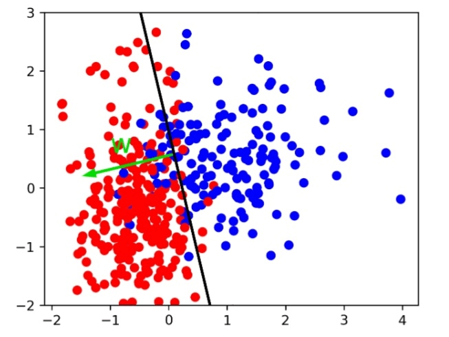
According to geometry, the formula indicates that a linear classifier's decision boundary will be a hyperplane in the feature space, where w is the normal vector of the plane. In this second example, red and blue are divided by a line. This classifier would categorize everything on the right side as blue and everything on the left side as red.

Questions? Again, obtaining the parameters w and b based on the training set constitutes the learning in this case, where the various algorithms vary. Many algorithms are available, and scikit-learn contains many, but we will cover the most popular ones.

Using the paradigm of empirical risk minimization that we discussed last time, finding parameters that minimize some loss o the training set is the simplest method to find w and b. When compared to regression, classification differs significantly in how we wish to measure misclassifications.

Rational Regression

The most popular linear classifier—and possibly the most popular classifier overall—is logistic regression. The goal is to represent the log-odds, which are represented above as log p(y=1|x) - log p(y=0|x), as a linear function. By rearranging the formula, you can model the logistic sigmoid, or p(y=1|x), as 1 over 1 +. It is shown here to the right. To describe a probability, the linear function wTx was essentially compressed between 0 and 1.

We wish to maximize the probability of the training set under this model given this equation for p(y|x). Maximum likelihood is the term for this strategy. You're looking for w and b such that they give the labels seen in the training data the highest probability. With a little rearrangement, you may arrive at this equation, which includes the log loss from the previous slide.

The class with the highest probability is the prediction. That is equivalent to asking whether the probability of class 1 is greater or less than.5 in the binary case. The probability of class +1 is exactly greater than.5 if the decision function wTx is bigger than 0, as can be seen from the logistic sigmoid plot. Therefore, determining the class with the greatest degree of certainty is equivalent to determining which side of the hyperplane provided by w we are on.

Okay, logistic regression is what this is. We achieve a w that defines a hyperplane by minimizing this loss. However, if you consider the last time, this is only a portion of what we wanted. This formulation doesn't care about coming up with a straightforward answer; instead, it strives to suit the training data.

Picking a loss?

y^=sign(wTx+b)
minw∈Rp,b∈R∑i=1n1yi≠sign(wTx+b)
.center[

To determine how well the given w and b fit the training set, we must create a loss function for them. Minimize the number of incorrect classifications or the 0-1 loss, but note that this loss is non-convex, discrete, and difficult to minimize. As a result, we must relax it, which means we need to identify an upper convex bound for this loss. This is carried out on the inner product wTx, commonly known as the decision function, rather than the actual forecast. In this graph, the loss for class 1 is represented by the inner product on the x-axis.

The hinge loss and the log loss comprise most of the other losses we'll discuss. Although they are both continuous and convex, it is clear that they are both upper bounds on the 0-1 loss. Both of these losses are concerned with "how correct" your prediction is or how positive or negative your decision function is, in addition to the fact that you make an accurate prediction. Beginning with the logistic loss, we'll go into greater detail regarding the reasons for these two losses.

Classifiers with multiple levels

There is to know about the two loss functions and regularisation. Hopefully, you now understand how these two classifiers operate and can see they are similar in use.

The transition from binary classification to multi-class classification is what I want to examine next. There are two approaches: one is straightforward but clumsy, and the other is a little more intricate but theoretically sound.