Decision Tree in Python

Decision Tree is one of the most essential algorithms in the area of machine learning for classification and regression.

But let us first talk about the lifespan of every machine learning model before starting with the method. This graphic illustrates the development of a scratch model for machine learning, then follows up the same model with hyperparameter tuning, determines the implementation methods for that model and establishes logging and monitoring frameworks once implemented.

Decision tree method is one of the most flexible machine learning algorithms that can analyse both regression and classification. It works extremely strong and with complicated datasets. It's pretty straightforward to comprehend, besides that. This method works by splitting the entire data set into a tree-like structure depending on specific criteria and circumstances.

Take a simple example, say it is Friday evening and you can't decide whether to go home or remain. Let it decide for you through the decision tree.

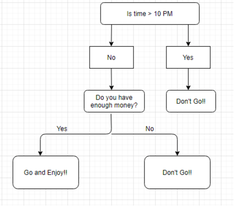
• The node will be selected depending on a certain circumstance, e.g. when our root node is >10 pm.
• The root node was then divided into children's notes according to the provided criteria. In the previous illustration the right child node met the requirement and there were no more questions.
• The left node of the kid did not fulfil the criterion and was thus divided into another condition.
• The procedure will continue until all requirements have been satisfied, or if you have already determined the depth of your tree, e.g. the depth of our tree, 3.

Decision Tree for Regression

When regression is performed using a decision tree, we are trying to split the X values into separated and uncomplicated areas for example for a set of potential values X1, X2, ..., Xp; we are going to attempt to divide them into J distincted and uncomplicated areas R1, R2, . – RJ. For a particular observation that falls within the RJ area, the forecast is the mean of the y-response values for each observation(s) of the training in the Rj region. The R1,R2, . ., RJ areas are chosen to decrease the following sum of residual squares:

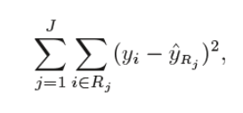
Where yrj is the mean of all variables of response in area 'j' (second term).

As indicated above, we attempt to divide X values into j areas, however in computing time it is highly costly to attempt to fit each set of X values into j regions. Recursive binary split (Greedy method). Thus, a decision tree opts for a gullible method at the top down in which nodes are divided into two regions according to the provided criteria. This means that not every node is divided but those that fulfil the requirement are divided into two branches. It is considered greedy because at that moment it splits best instead of trying to divide one step towards a better tree in the next stages. It determines to divided the observations into various regions(j) by a threshold value(s) such that the RSS is minimal for Xj>=s and Xj <s.

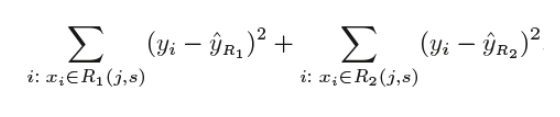
For this equation, j and s are determined to have the smallest value in this equation. Based on this s and j value, the areas R1, R2 are selected, so that the above equation has the lowest value. More regions are also divided amongst the above-mentioned zones, depending on the same logical criteria. This runs until a (pre-defined) stop criteria is met. The forecast is made on the basis of the mean of data in this region once all regions are divided.

The aforementioned procedure is highly likely, given that it is quite complicated, to overfit the training data.

Shape of the Tree

Tree cuttings are a way to minimise the complexity and variation of data by cutting the tree down to the entire tree (obtained in the previous procedure). We may regularise the decision tree model by adding a new term just as we regulated linear regression.

Where T is the subset of the entire T0 tree And α is the non-negative parameter which impairs the MSE by increasing the length of the tree. By utilising cross-validation, these α and T values are determined, the lowest test error rate is provided by our model. This is how the model of the decision tree is working. Let's now look at the functioning algorithm of a decision tree classification. Algorithm of greedy The greedy algorithm "searches for an optimum breach at top level according to Hands-on Machine Learning Book, then repeats the procedure at each level. It does not verify that the split leads to many levels of impurity at the lowest feasible level.

• Criterion: (default="gini") string, discretionary.
• The quality estimation capacity of a division. "gini" for Gini debasements and "entropy" are upheld basis for acquiring data.
• Max profundity: int or none (default=none) discretionary Tree's most elevated profundity. Assuming none, the hubs are stretched out to simply every one of the leaves, or to not as much as min tests split examples in every one of the leaves.
• Min tests split (default=1): int, drift, discretionary. The insignificant number of tests essential for isolating an inner hub:
• If int, consider the insignificant number for min tests split.
• If drifting, the base number of tests for each split is a small portion, and roof is (min tests split * n tests). Changed adaptation:: 0.18 Float portion esteems added.
• msamples leaf (default=1): int, coast, discretionary. The base example number essential for a leaf hub. A split point is possibly viewed as in a profundity in the event that it leaves tests of preparing min tests leaf in each part of the left and right. This can smooth the example, specifically during relapse.
• If int, the base number ought to be min tests leaf.
• If drift, min tests leaf will comprise of a level of the hub, and the base examples for every hub will approach the roof (min tests leaf*n tests).
• Max highlights (default=None): int, buoy, string or None When searching for the best separation, the measure of elements to analyze is:

If int, then consider `max_features` features at each split.

If float, then `max_features` is a fraction and

`int(max_features * n_features)` features are considered at each split.

   - If "auto", then `max_features=sqrt(n_features)`.

   - If "sqrt", then `max_features=sqrt(n_features)`.

   - If "log2", then `max_features=log2(n_features)`.

   - If None, then `max_features=n_features`.

Note: The split pursuit doesn't end until something like one legitimate hub test parcel is distinguished, regardless of whether more than max include highlights should be viably investigated.

• Random state: int, RandomState or None (default=None) Instance, discretionary If the arbitrary state is the seed the generator utilizes, then, at that point, Random state is the irregular number generator if the RandomState occurrence is; If None, the RandomState object utilized by np.random is the arbitrary number generator.
• (Default=1e-7) min pollutions split: coast early stop limit for the development of the tree. In the event that the hub is over the limit, it will part, else it will be a leaf.
• Class weight: dict, rundown of dicts, "balance" or "none" Weights in the structure {class name: weight} associated with the classes. All classes ought to be weight one, if not expressed. A rundown of dicts can be displayed in a similar request for multi-yield issues as the y segments: bool, discretionary (default=False)
• Whether to recommend the information to speed up the quest for ideal parts. Setting this to genuine can dial back the preparation cycle for default sets of a choice tree on huge datasets. This can speed up preparing while using either a more modest dataset or a restricted profundity.
• When tuning the hyperparameters, we plan to recognize these hyperparameter sets and qualities that offer us a model with the best conceivable accuracy. Allow us to keep on upgrading our model.

In[]:

scalar = StandardScaler()

x_transform = scalar.fit_transform(X)

In[]:

x_train,x_test,y_train,y_test = train_test_split(x_transform,y,test_size = 0.30, random_state= 355)

Although our dataset is tiny, let us apply PCA to choose a feature and see whether our accuracy is improved.

In []:

from sklearn.decomposition import PCA

import numpy as np

pca = PCA()

principalComponents = pca.fit_transform(x_transform)

plt.figure()

plt.plot(np.cumsum(pca.explained_variance_ratio_))

plt.xlabel('Number of Components')

plt.ylabel('Variance (%)') #for each component

plt.title('Explained Variance')

plt.show()

We can observe that 8 components explain around 95 percent of the variation. So let's utilise these 8 main components instead of all 11 columns as input into our algorithm.

In [170]:

pca = PCA(n_components=8)

new_data = pca.fit_transform(x_transform)

principal_x = pd.DataFrame(new_data,columns=['PC-1','PC-2','PC-3','PC-4','PC-5','PC-6','PC-7','PC-8'])

In []:

principal_x

Post-Pruning

Post-pruning is the process of first generating the decision tree and then deleting the non-important branches. Cross-validation data is utilized to assess whether or not extending a node improves the effect of pruning and testing. If there is an improvement, this node is further extended if the precision decreases, then the node must not be expanded and converted to a leaf node.

Pre-pruning

Pre-pruning, known as forward pruning, prevents the generation of non-important branches. It utilises a criterion to determine when splitting certain branches should end prematurely when the tree is produced.

Classification Trees

For quantitative data, regression trees are employed. We utilise classification trees for qualitative data or categorical data. We divide the nodes in regression trees based on RSS criteria, while the classification is based on the error rate of classification, the impurity of Gini and entropy. Let's be detailed in these words.

Entropy

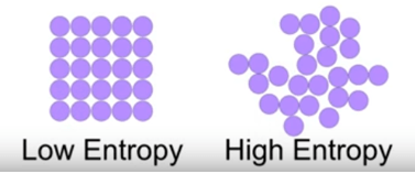
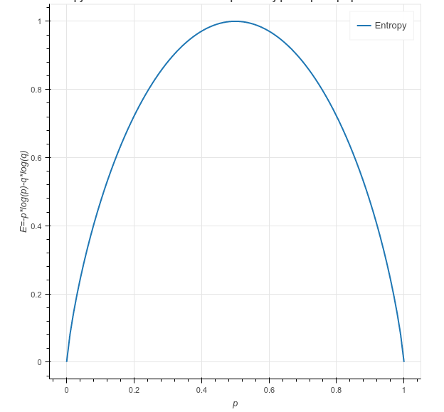
Entropy is the randomness measurement for the data. In other words, the impurity in the dataset is given. When we split our nodes into two areas and place distinct observations in both regions, the primary objective is to reduce entropy, i.e. to minimize randomness in the region. When dividing the node doesn't contribute to a reduction in entropy, we try to divide or halt according to another criterion. A area is clean when it includes data on identical labels (low entropy) and random if a label mix is present (high entropy). Suppose 'm' observations are present and we must classify them according to categories 1 and 2.

Let's assume, there are 'n' observations in category 1, and 'm-n' observations in category 2.

p= n/m and q = m-n/m = 1-p

Then, entropy for the given set is:

E = -p*log2(p) – q*log2(q)

In category 1 all observations are p = 1 and all observations are category 2, then p = 0, both of them E =0, as the categories have no randomness. When half of the data are in categories 1 and half in category 2, then a maximum entropy is p = 1/2 and q = 1/2. E = 1.

Information Gain

The gain of information calculates the entropy drop when the node is divided. It is the difference between entropies before and following the division. The more information is gained, the greater the entropy.

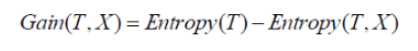
Where T is the pre-divided node and X is the T divided node.

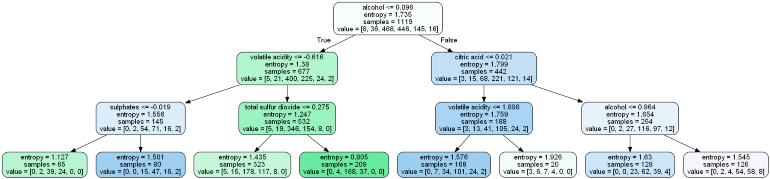
A tree divided by entropy and the value of information looks like:

Ginni Impurity

According to wikipedia, "gini impurity is a measure of how often a randomly selected item in the set is wrongly labelled by random label distribution in a subset." The probability is computed by multiplying the classification of one observation by sum of all probabilities and classifying it in the wrong class. Let's assume that there are k classes and that an observation comes in class I.

The impurity value for ginni falls between 0 and 1.0 is no uncleanness and 1 is random. The root node to divide is the node for which Ginni impurity is less common.

A tree divided according to the impurity value of ginni seems like:

Different Algorithms for Decision Tree

• ID3: it's one of the algorithms that are used to create the classification decision tree. It leverages the acquisition of information to locate and divide root nodes. Only categorical characteristics are accepted.
• C4.5: is a continuous, as well as a distinct, value extension of ID3 and superior than ID3 algorithms. It is often used for grading reasons.
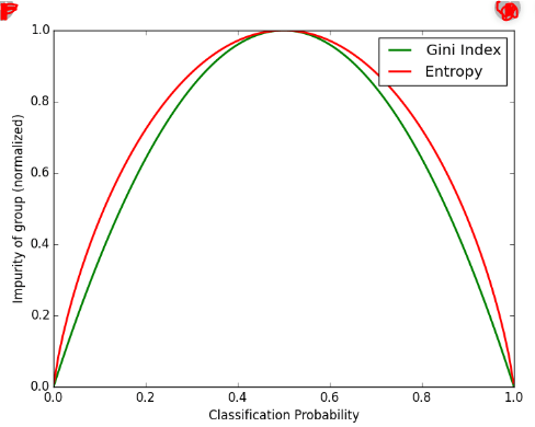
• Algorithm for classification and regression (CART): This method is the most frequent utilized for building decisive trees. It utilizes Gini impurity to calculate root nodes by default, but "entropy" may be used for criterion. This technique works on issues of both regression and classification. In our python implementation, we will utilize this algorithm.

The impurity of Entropy and Ginni can be reversibly utilised. It has no great impact on the result. Ginni can be computed more easily than entropy, because entropy includes a computation of the log term. Therefore, Ginni is the default algorithm for the CART algorithm. We can observe that there is not much difference between them when we are plotting ginni vs entropy:

Decision Tree advantages:

• It may be used both for issues of regression and classification.
• Decision Trees are relatively straightforward to understand because the splitting rules are explicitly indicated.
• When you envision complex decision tree models, they are extremely easy. It is only visualized that can be comprehended.
• There is no requirement for scaling and normalization.

Disadvantages of Decision Tree:

• During the greedy method, a little change of data may lead to model instability.
• For decision trees, the likelihood of overfitting is quite high.
• It takes longer than other classification methods to train the model for the decision tree.

Cross-Validation

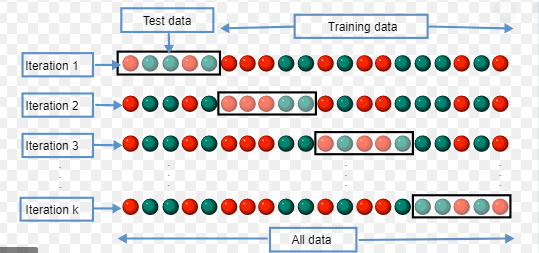
Suppose you are using a certain algorithm to train a model on a given data set. You attempted to find the precision of the trained model using the same training data and discovered that it was 95% or maybe 100% accurate. What does that mean? What does that mean? Is your model predictable? The reply is no. Why? Because the model has trained on the particular data, i.e. the data is well-known and generalized. But if you try to forecast a fresh piece of information, it most likely gives you very low accuracy, as it has never seen the data before. That's the overfitting problem. Cross-validation enters the picture in order to address this problem. Cross-validation is a re-evaluation approach with the essential notion that the training data set should be divided into two portions, namely training and testing. You try to train the model on one portion (train), and on the second part (test), i.e. the data that is not visible for the model, to forecast and verify your model. If your model works on your test data in a decent manner, it implies that you have not over fitted the training data and can trust the prediction, but our model is not to be believed if it is performed with bad precision, we must adjust our algorithm.

See the many Cross-Validation approaches:

Method Hold Out:

The techniques of the CV are the most fundamental. The dataset is simply divided into two training and test sets. The training dataset is utilized for training the model and the test data for predictions are then included in the learned model. This is the basis for checking and evaluating our model. The approach is utilised since it is less expensive computer-based. However, the assessment based on the Hold-out set might have a significant variability, because the data points in the training set and the test data rely substantially on. Whenever this division changes, the assessment will be different.

• k-fold Cross-Validation

Implementation in Python

For implementing decision tree algorithms, we will utilise the Sklearn module. Sklearn employs the CART method and uses Gini impurity as a standing criterion in the division of nodes by default.

Importing required Modules

import pandas as pd

import graphviz

from sklearn.tree import DecisionTreeClassifier, export_graphviz

from sklearn import tree

from sklearn.model_selection import train_test_split,GridSearchCV

from sklearn.preprocessing import StandardScaler

from sklearn.metrics import accuracy_score, confusion_matrix, roc_curve, roc_auc_score

from sklearn.externals.six import StringIO

from IPython.display import Image

from sklearn.tree import export_graphviz

import pydotplus

data = pd.read_csv(“winequality_red.csv”)

data

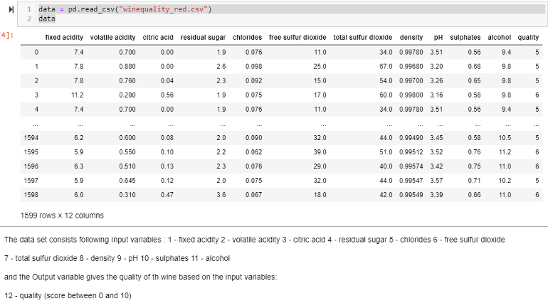
X = data.drop(columns = 'quality')

y = data['quality']

where X is Independent values and y is dependent values

Splitting dataset into Test data and Training data

x_train,x_test,y_train,y_test = train_test_split(X,y,test_size = 0.30, random_state= 355)

In []:

#let's first visualize the tree on the data without doing any pre processing

clf = DecisionTreeClassifier()

clf.fit(x_train,y_train)

Out[]:

DecisionTreeClassifier(class_weight=None, criterion='gini', max_depth=None,

                       max_features=None, max_leaf_nodes=None,

                       min_impurity_decrease=0.0, min_impurity_split=None,

                       min_samples_leaf=1, min_samples_split=2,

                       min_weight_fraction_leaf=0.0, presort=False,

                       random_state=None, splitter='best')

# create a dot_file which stores the tree structure

dot_data = export_graphviz(clf,feature_names = feature_name,rounded = True,filled = True)

# Draw graph

graph = pydotplus.graph_from_dot_data(dot_data)

graph.write_png("myTree.png")

# Show graph

Image(graph.create_png())

Let the tree above be understood:

The first value specifies a column and the selecting and splitting condition of the root node.

The second value gives a number of observations in the node value within the square brackets of gini impurities for the selected node samples, i.e. in the above figure, 8 observations are of class 1, 38, clase 2, 468 of class 3 and so on, which means that the node value is present at that time in the square brackets.

In[]:

clf.score(x_train,y_train)

Out[]:

1.0

In []:

py_pred = clf.predict(x_test)

In[]:

# accuracy of our classification tree

clf.score(x_test,y_test)

Out[]:

0.5791666666666667

No pre-processing of our data and no hyperparameter tweaking have now been carried out.

Let's all do that and see what increases our score.

What are hyper parameters?

We can see below the decision tree classifier algorithm takes all those parameters which are also known as hyperparameters.

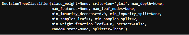
Let's look at the parameters most important (as per sklearn documentation)