Python - Binomial Distribution

Introduction

Definition of the Binomial Distribution

The method of counting how many instances of a specific event there have been is called the binomial distribution. It will outline the possible outcomes or possible scenarios for the certain occurrences that will result in the certain numbers. Statistics on counts or may be how many times an event occurs are frequently analyzed in this binomial distribution.

Data Science using Binomial Distribution

We have only recently learned about the binomial distribution. According to data science, the binomial distribution definition remains the same. It can be explained as the other kind of discrete distribution that is a binomial distribution. Wherever a series of Bernoulli trials are being observed, the binomial distribution appears. Thus, the Bernoulli distribution is what we refer to if we just have one trial. However, if there are several trials, we must consider a binomial distribution.

Python and the Binomial Distribution

Binomial distribution is illustrated using Python. We already know that when a random experiment has more than one trial, we consider the binomial distribution. In this binomial distribution, the answer will be in the form of yes or no.

Python's binomial distribution provides us with information on the likelihood that n separate trials will be successful. These tests ask yes-or-no questions. Tossing a coin is a possible illustration.

The binomial distribution in probability theory has two parameters, n and p.

To satisfy binomial distribution, there must be some conditions. When the probability distribution satisfies the following conditions, it becomes a binomial probability distribution.

Conditions

• There must be a specific number of trails.
• Each trial's results must be distinct from one another.
• Additionally, each trial's likelihood success rate must remain constant.
• Each trial may only yield two results, or results that can be reduced to two results. Success or failure might arise from these findings.

Binomial Distribution formulae

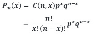
The probability distribution function P(x) of binomial distribution is given by

P(x) = [n! / x! (n-x)!] _· p^x (1 - p)^n-x

Where, in the formula the terms 

n = The overall number of incidents.

x = Total number of successful events, r (or) x.

p = Chance of success on a single attempt.

1 – p  = Probability of failure = q

and  n Cr equals [n! /r! (nr) ]

Example

Let's look at a sample issue. The following is an illustration of the binomial distribution:

In a random experiment, a coin is taken for tossing and it was tossed exactly 10 times. what are the probabilities of obtaining exactly six heads out of total 10 tosses?

The binomial distribution table will provide the likelihood of x successes for each conceivable value of x if "getting a head" is regarded as a success.

x	p(x)
0	0.00097
1	0.00976
2	0.04394
3	0.11718
4	0.20507
5	0.24609
6	0.20507
7	0.11718
8	0.04394
9	0.00976
10	0.00097

Now we can find the answer for the above question by checking the p(x) values in the distribution table. According to the question, When a coin is tossed 10 times, there is a 0.20507 chance of receiving exactly 6 heads.

Drawing Plots & Graphs using Python

To get the illustration of the binomial distribution table for the above problem we can use python programming language. By writing code in python, we can easily analyze the distribution. And along with that we can plot graphs for easier interpretation.

To get this job done we need some predefined modules of python. They are Matplotlib and SciPy respectively. Where SciPy is used for determining the distribution table and matplotlib is for plotting graphs.

Matplotlib Module

Python's Matplotlib is a fantastic visualizing package that is simple to use. A cross-platform library called t is used to create 2D plots from arrays of data. NumPy, Python's extension for numerical mathematics, is used by Matplotlib, which is built in Python. It offers an object-oriented API that facilitates the integration of charts into programs utilizing Python GUI toolkits.

SciPy Module

SciPy is a scientific library for Python. The NumPy library, which offers simple and quick dimensional array manipulation, is a prerequisite for the SciPy library. The SciPy library was created primarily so that it would be compatible with NumPy arrays. It offers a variety of simple and effective numerical techniques, including methods for numerical integration and optimization.

Distribution table using Python SciPy Module

Code

from scipy.stats import binom
# initializing the values of both p and n
n = 10
p = 0.5
# determining the x values
x_val = list(range(n + 1))
# the pmf values li
dist = [binom.pmf(x, n, p) for x in x_val ]
# to print the distribution table
print("x\tp(x)")
for i in range(n + 1):
	print(str(x_val[i]) + "\t" + str(dist[i]))
# to get the values of mean and variance
m, v = binom.stats(n, p)
#now print both mean and variance values respectively
print("mean is "+str(m))
print("variance is "+str(v))

Output

x	p(x)
0	0.0009765625
1	0.009765625000000002
2	0.04394531250000004
3	0.1171875
4	0.2050781249999999
5	0.24609375000000003
6	0.2050781249999999
7	0.11718749999999999
8	0.04394531249999997
9	0.009765625000000002
10	0.0009765625
mean is 5.0
variance is 2.5

Graph using Matplotlib module

Code

from scipy.stats import binom
import matplotlib.pyplot as plt
# initializing the values of both p and n
n = 10
p = 0.5
# determining the x values
x_val = list(range(n + 1))
# the pmf values list
dtable = [binom.pmf(x, n, p) for x in x_val ]
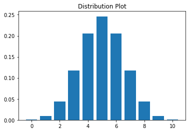
# plotting the graph
plt.title("Distribution Plot")
plt.bar(x_val, dtable)
plt.show()

Output

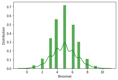
Distribution Table with the help of Seaborn Module

To generate these probability distribution graphs, we use the built-in methods of the Seaborn Python module. The scipy software also aids in the production of the binomial distribution.

Code

import seaborn
from scipy.stats import binom
d =binom.rvs(n=10,p=0.5,loc=0,size=1200)
ax=seaborn.distplot(d,
                kde=True,
                color='green',
                hist_kws={"linewidth": 30,'alpha':0.66})
ax.set(xlabel='Binomial',ylabel='Distribution')

Output

[Text(0.5, 0, 'Binomial'), Text(0, 0.5, 'Distribution')]