Python Linear regression

In this tutorial, we will understand the meaning, usage, and types of Linear Regression. Further, we will comprehend the terms cost function and Optimization.

Linear Regression is the widely used Machine Learning algorithm. It comes under Supervised Learning. It is an arithmetical technique employed for the predictive study. It estimates real, continuous, or numeric variables such as sales, income, price of any item, etc.

The Linear regression algorithm displays a linear association between dependent variable y and one or more sovereign (x) variables; hence it is called linear regression.  The linear association is depicted in a Linear regression which illustrates the way in which the value of one dependent variable alters with the other independent one.

Graphically, the straight line is employed to indicate the relationship between the variables.

The straight line in the graph shows the mark of regression.

Mathematically, the linear relationship is denoted as:

y= a0 + a1x + c

Here,

Y= Dependent Variable that acts as our target Variable.
X= Independent Variable that acts as our forecaster Variable.
a0= Intercept of the line which provides an extra degree of freedom.
a1 = Coefficient of Linear regression.
c = chance of fault.

Here, X and Y values are considered for the training dataset.

Line of Regression

Now, let us deal with the line of regression.

A line of regression is the one that displays the relationship between the independent and dependent variables.

1. Positive Linear relationship:

Positive Linear relationships are those in which the value of the dependent variable increases on the Y-axis and the value of an independent variable increases on the X-axis 

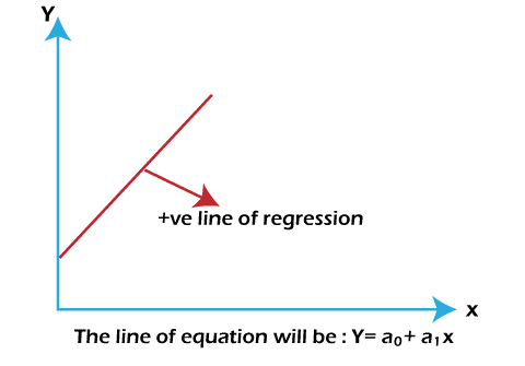
Here, the line equation is: a₀ + a₁x + c

2. Negative Linear relationship:

Negative Linear relationships are those in which the value of the dependent variable decreases on the Y-axis and the value of an independent variable increase on the X-axis.

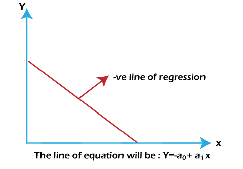
Here, the line equation is: - a₀ + a₁x + c

Types of Linear Regression:

There exist two types of linear regression.

1. Simple Linear Regression

The value of a mathematical dependent variable is predicted with the aid of a single independent variable in a simple Linear Regression.

2. Multiple Linear Regression

The value of a mathematical dependent variable is predicted with the aid of multiple sovereign variables in multiple linear regression.

The best fit line:

The chief area is to find the finest suitable line while dealing with linear regression. It means that there should exist minimum fault between predicted values and actual values. Hence, the best fit line will have the smallest amount of error.

Cost function:

1. The dissimilar values of the coefficient of lines (a₀, a₁) give a dissimilar line of regression. Thus, we need to compute the best values for a₀ and a₁ to find the best fit line, Hence, the cost function is employed for the calculation of the best fit line.
2. The Cost function calculates the performance of a linear regression model and thus improves the regression coefficients or weights.
3. To calculate the exactness of the mapping function, the cost function can be employed which plots the input variable to the resultant variable. The hypothesis function is the other name of the mapping function.

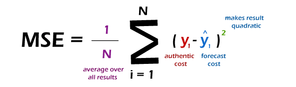
Mean Squared Error (MSE) cost function

The Mean Squared Error (MSE) cost function is employed to calculate the cost function of linear regression. It is the midpoint of squared error arising between the predicted values and actual values.

It can be written

Here,

N = Overall quantity of observations
Yi = Authentic cost
(a1x_i+a₀) = Forecast cost.

Optimization

Optimization is the process of discovering the best model out of several models and the process of determining the way by which a line of regression fits the group of observations is known as the Goodness of Fit.

R-squared method:

It is a mathematical way employed for the computation of the goodness of fit.

Here, the value lies between 0 and 1 which in turn denotes the percentage.

The good value depends on the domain we are working in. But it should neither be too high nor too low.  0.8 is considered a great value in many areas.

The coefficient of determination is considered for simple linear regression and the coefficient of multiple determination is considered for multiple linear regression.

The calculation formula is:

R-squared = Totality of squares of residuals/ Sum of squares