Multiple Linear Regression using Python

Linear Regression:

Linear regression is a method that models the relationship between a dependent variable and one or more independent variables; in other terms, that models the relationship between a target variable and simple regression or multiple regression.

This model assumes a relationship between the given inputs and the output variables. We can also determine the coefficients required by the model to predict the new data.

Linear regression is of two forms; they are

• Simple Linear Regression
• Multiple Linear Regression

Simple Linear Regression:

Simple linear regression (SLR) predicts a response using a single feature or variable. In simple linear regression, all the variables are linked linearly. Here the main purpose is to find a linear equation used to predict the answer value of y concerning the feature or the independently derived variable (x).

Below is a dataset with x features and y responses respective to x.

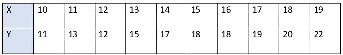
For simple understanding, we define

X as features, that is x = [10, 11, 12, ……, 19],

Y as response, that is y = [11, 13, 12, ……, 22]

We have considered 10 values in the above table

The graphical representation of the above dataset looks like this:

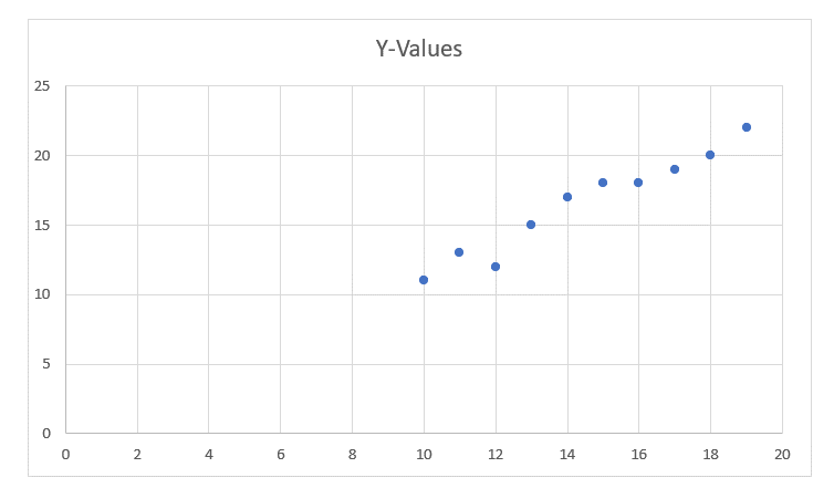
After this, we have to find or identify the most suitable line for this scatter graph to find the response of any new value for a feature.

This line is referred to as the regression line. We have some equations of the regression line.

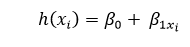
Here,

• h(x_i) is the predicted response value for the i^th.
• β₀  and β_1xi are regression coefficients.

If we want to build the model, we must know how to estimate the value of regression coefficients. If we know how to estimate regression coefficients, then only we can use this model to get the responses.

Concept of Least Squares:

Y_i = ₀ + Ρ_1xi + Ρ_i = h(x_i) + Ρ_i Ρ Ρ_i = y_i – h(x_i)

Here, Ρ_i is a residual error in i^th observation.

So, we have to minimize the total residual error.

The cost function or squared error, b as:

b(β_0, β₁) = 1/2nΣⁿ_{I = 1} έ²_i

We have to find the values of Ρ₀ and Ρ₁  to find b(Ρ₀ and Ρ₁) minimum.

Let us not go into deep calculations. We are presenting the result below:

β₁ = SS_ab / SS_aa

β₀ = b – β₁a

where SS_ab would be the sum of cross deviations of “b” and “a”:

SS_ab = Σⁿ_{I = 1} (a_i – a)(b_i – b) = Σⁿ_{I =1} b_ia_i – nab

And SS_aa would be the sum of squared deviations of “a.”

SS_aa = Σⁿ_{i = 1}(a_i – a)² = Σⁿ_{i = 1}a_i² – n(a)²

Modules used:

• Numpy
• Pandas
• Matplotlib
• Sklearn

Example:

#simple program for simple linear regression
import numpy as np  
import matplotlib.pyplot as mtp  
  
def estimate_coeff(p, q):  
# Here, we will assume the total number of points or observation  
    n1 = np.size(p)  
# Now, we will calculate the mean of a and b vector  
    p = np.mean(p)  
    q = np.mean(q)  
  
# here, we will calculate the cross deviation and deviation about a  
    SS_pq = np.sum(q * p) - n1 * q * p  
    SS_pp = np.sum(p * p) - n1 * p * p  
  
# here, we will calculate the regression coefficients  
    b1 = SS_pq / SS_pp  
    b0 = q - b1 * p  
  
    return (b0, b1)  
  
def plot_regression_line(p, q, b):  
# Now, we will plot the actual points or observations as a scatter plot  
    MTP.scatter(p, q, color = "m",  
            marker = "o", s = 30)  
  
\# here, we will calculate the predicted response vector  
    q_pred = b[0] + b[1] * p  
  
# here, we will plot the regression line  
    mtp.plot(p, q_pred, color = "g")  
  
# here, we will put the labels  
    mtp.xlabel('p')  
    mtp.ylabel('q')  
  
# here, we will define the function to show plot  
    mtp.show()  
  
def main():  
# entering the observation points or data  
    p = np.array([10, 11, 12, 13, 14, 15, 16, 17, 18, 19])  
    q = np.array([11, 13, 12, 15, 17, 18, 18, 19, 20, 22])  
  
# now, we will estimate the coefficients  
    b = estimate_coeff(p, q)  
    print("Estimated coefficients are :\nb0 = {} \  
        \nb_1 = {}".format(b[0], b[1]))  
  
# Now, we will plot the regression line  
    plot_regression_line(p, q, b)  
  
if __name__ == "__main__":  
    main()  

Output:96

Estimated coefficients are:
b0 = -0.5606006069
b1 = 1.17696867686

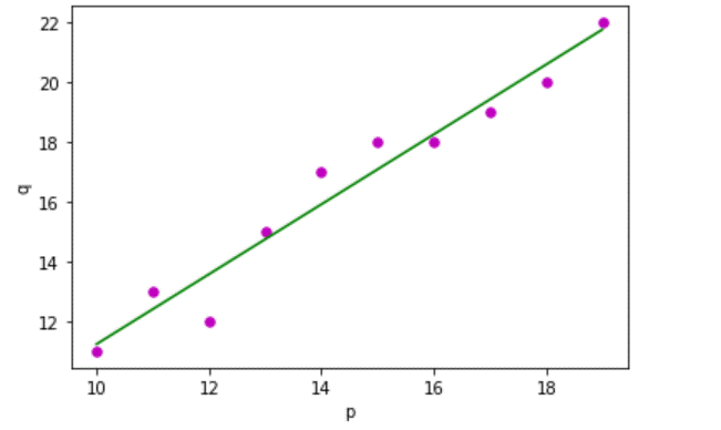
As we can see from the output, we have drawn simple linear regression using Python and the modules matplotlib used to plot the graph and the numpy module.

Multiple Linear Regression:

We require only one independent variable as the input in simple linear regression. However, we provide multiple independent variables for a single dependent variable in multiple linear regression. It is a Machine learning algorithm.

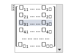
Q(Feature Matrix) = Q is a matrix of size "a * b" where "Q_ij" represents the values of the j^th attribute for the i^th observation.

We represent in the matrix form.

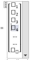
S (Response Vector) = It is a vector of size “a” representing the response value for the i^th observation.

“A” regression line is:

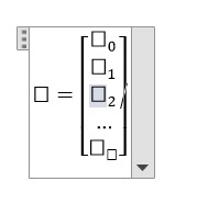
  h(Q_i) = β₀ + β_1qi1 + β_2qi2 + β_3qi3 + β_4qi4 + β_5qi5 +………. + β_bqib

Here, h(q_i) is known as the response value for the i^th observation point. We have to find the regression coefficients that are Ρ₀, Ρ₁, Ρ₂……, Ρ_b .

We have another formula:

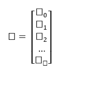
S_i = β₀ + β_1qi1 + β_2qi2 +β_3qi3 + ……..+β_bqib +Є_i

We can represent the linear model in matrix form

Here,

And,

Using the Least Squares algorithm, we can get the estimated value of b (b^’). We can only use the Least Squares method when the residual error is minimised.

The result will be shown as

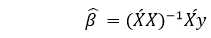
Here, (‘) represents the transpose of the matrix and -1 represents the reverse of a matrix.

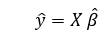
The above formula is used for calculating the multi-linear regression model. Here Y’ is the calculated response vector.

Example:

//program for multiple linear regression using Python
import matplotlib.pyplot as mtp 
import numpy as np  
from sklearn import datasets as data
from sklearn import linear_model as lmd  
from sklearn import metrics as mt  
  
# First, we will load the Boston dataset  
boston1 = data.load_boston(return_X_y = False)  
  
# Here, we will define the feature matrix(H) and response vector(f)  
H = boston1.data  
f = boston1.target  
  
# Now, we will split X and y datasets into training and testing sets  
from sklearn.model_selection import train_test_split as tts  
H_train, H_test, f_train, f_test = tts(H, f, test_size = 0.4,  
                                                    random_state = 1)  
  
# Here, we will create a linear regression object  
reg1 = lmd.LinearRegression()  
  
# Now, we will train the model by using the training sets  
reg1.fit(H_train, f_train)  
  
# here, we will print the regression coefficients  
print('The Regression Coefficients are: ', reg1.coef_)  
  
# Here, we will print the variance score: 1 means perfect prediction  
print('The Variance score is: {}'.format(reg1.score(H_test, f_test)))  
  
# Here, we will plot for residual error  
  
# here, we will set the plot style  
mtp. style.use('five thirty eight')  
  
# here, we will plot the residual errors in training data  
mtp.scatter(reg1.predict(H_train), reg1.predict(H_train) - f_train,  
            color = "green", s = 10, label = 'Train data')  
  
# Here, we will plot the residual errors in test data  
mtp.scatter(reg1.predict(H_test), reg1.predict(H_test) - f_test,  
            color = "blue", s = 10, label = 'The Test data')  
  
# Here, we will plot the line for zero residual error  
mtp. hlines(y = 0, xmin = 0, Xmax = 50, linewidth = 2)  
  
# here, we will plot the legend  
mtp.legend(loc = 'upper right')  
  
# now, we will plot the title  
mtp.title("The Residual errors")  
  
# here, we will define the method call for showing the plot  
mtp.show()  

Output:

The Regression Coefficients are:  [   -8.95714048e-02  6.73132853e-02  5.04649248e-02  2.18579583e+00       -1.72053975e+01  3.63606995e+00  2.05579939e-03 -1.36602888          2.89576718e-01      -1.22700072e-02         -8.34881849e-01  9.40360790e-03      -5.04008320e-01    ]


The Variance score is: 0.7209056672661751

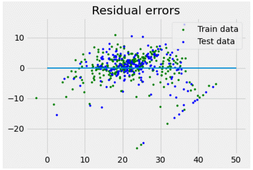
As we can see the output of the program how we have drawn the multiple linear regressions using Python. In the program, we have imported the modules matplotlib, numpy, and sklearn. Matplotlib is used to plot the graph and represent the graph on the output screen. Sklearn for dataset usage and numpy for the larger arrays of the dataset.