Logistic Regression in Python
What is Logistic Regression?
It is a method used in the case of a definite dependent (target) variable. It is used for classifying problems and prediction. For example, fraud detection, spam detection, etc.
User Database:
It is a dataset that is used to store information about users from a company’s database. Information like User ID, Age, Gender, Purchase, and Estimated Salary. We will be using this database to predict whether the user will be purchasing the newly launched product or not.
We will be referring to the below-given table to see from where the data is being fetched:
| User ID | Gender | Age | Estimated Salary | Purchased |
| 15624510 | Male | 28 | 89000 | 1 |
| 15798535 | Male | 34 | 74000 | 0 |
| 16583456 | Male | 24 | 154000 | 1 |
| 15324584 | Female | 27 | 24000 | 0 |
| 15498856 | Female | 45 | 32000 | 0 |
| 15478996 | Male | 36 | 94000 | 1 |
| 16875569 | Male | 47 | 120000 | 1 |
| 17854685 | Female | 25 | 58000 | 0 |
| 16542586 | Female | 51 | 44000 | 0 |
| 17845904 | Female | 18 | 25000 | 0 |
| 18745985 | Male | 19 | 52000 | 0 |
| 13566429 | Female | 30 | 64000 | 0 |
| 14459876 | Female | 23 | 62000 | 0 |
| 12354892 | Male | 31 | 84000 | 1 |
| 14689992 | Male | 49 | 72000 | 0 |
| 14566258 | Female | 36 | 60000 | 0 |
| 19886523 | Male | 24 | 85000 | 1 |
| 14566288 | Male | 20 | 64000 | 0 |
| 17955568 | Male | 39 | 38000 | 0 |
| 19547624 | Female | 41 | 18000 | 0 |
Now, let us make a logistic regression model to predict about the user will purchase the new item or not.
#Importing Libraries to be used:
import numpy as nps
import matplotlib.pyplot as plts
import pandas as pds
Reading and exploring the data:
data_set = pds.read_csv("User_Data.csv")
Age and Estimated Salary are the two factors that have to be noticed to predict the outcome of the event, here, gender and User ID are not to be considered.
# Input
a = data_set.iloc[ : , [1, 4] ].values
# Output
b = data_set.iloc[:, 5].values
Splitting the Dataset: Test and Train Dataset
The dataset is split to train and test. 25% of the data is used to test the data and the remaining 75% is used to train the data for the performance of the model.
from sklearn.model_selection import train_test_split
x_train, x_test, Y_train, Y_test = train_test_split(a, b, testsize = 0.25, randomstate = 0)
After this step, we have to make sure that the feature scaling has been performed, as values of both “Estimated Salary” and “Age” lie in a different range. If this step is not taken then the “Estimated Salary” feature will single-handedly dominate the “Age” feature when in the data space, the model will be searching for the nearest neighbor to the data point.
Example to illustrate feature scaling function:
from sklearn.preprocessing import StandardScaler
from sklearn.model_selection import train_test_split
data_set = pds.read_csv("User_Data.csv")
# Input
a = data_set.iloc[ : , [1, 4] ].values
# Output
b = data_set.iloc[ : , 5].values
from sklearn.model_selection import train_test_split
x_train, x_test, Y_train, Y_test = train_test_split(a, b, testsize = 0.25, randomstate = 0)
scx = StandardScaler( )
atrain = scx.fit_transform(atrain)
atest = scx.transform(atest)
print (atrain[ 0 : 15, : ] )
Note: Here the data_set stores the values given in the above table.
Output:
[ [ 0.58164944 -0.88670699]
 [-0.60673761 1.46173768]
 [-0.01254409 -0.5677824 ]
 [-0.60673761 1.89663484]
 [ 1.37390747 -1.40858358]
 [ 1.47293972 0.99784738]
 [ 0.08648817 -0.79972756]
 [-0.01254409 -0.24885782]
 [-0.21060859 -0.5677824 ]
 [-0.21060859 -0.19087153] ]
Explanation:
In this output, we can see that the values of both, i.e., “Age” and “Estimated Salary” are now scaled from “-1 to 1”, so now, both features can equally contribute to the decision-making.
Finally, now we can train our Logistic Regression model.
Training the Model:
from sklearn.linear_model import LogisticRegression
# Initialising a variable to hold the classified value
clsfi = LogisticRegression(random_state = 0)
clsfi.fit(atrain, btrain)
Now the model has been trained, after this, we will be using it for predictions on testing data.
b_prdct = clsfi.predict(atest)
Now we can check the performance of the model created by us, i.e., Confusion Matrix.
Evaluation of “metrics”:
from sklearn.metrics import confusion_matrix
cnf_mat = confusion_matrix(btest, b_prdct)
print ("Format of Confusion Matrix : \t", cnf_mat)
Output:
Format of Confusion Matrix :
 [ [65 3]
 [ 8 24] ]
Example to illustrate the accuracy of our model:
from sklearn.metrics import accuracy_score
print ("Accuracy of our model: ", accuracy_score(btest, b_prdct) )
Output:
Accuracy of our model: 0.89
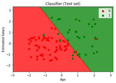
Another example to visualize the performance of our model:
from matplotlib.colors import ListedColormap
a_set, b_set = atest, btest
a1, a2 = np.meshgrid(np.arange(start = a_set[:, 0].min() - 1,
 stop = a_set[:, 0].max( ) + 1, step = 0.01 ),
 np.arange(start = a_set[:, 1].min( ) - 1,
 stop = a_set[:, 1].max( ) + 1, step = 0.01 ) )
plt.contourf(a1, a2, classifier.predict(
 np.array([a1.ravel( ), a2.ravel( ) ] ).T).reshape(
 a1.shape), alpha = 0.75, cmap = ListedColormap(('red', 'green')))
plt.xlim(a1.min( ), a1.max( ))
plt.ylim(a2.min( ), a2.max( ))
for x, y in enumerate(np.unique(b_set)):
 plt.scatter(a_set[b_set == y, 0 ], a_set[b_set == y, 1 ],
 z = ListedColormap( ('red', 'green') ) (x), label = y)
plt.title('Classifier (Test set)')
plt.xlabel('Age')
plt.ylabel('Estimated Salary')
plt.legend()
plt.show()
Output: