Hypothesis Testing in Python

Hypothesis Testing in python is widely used along with statistics.

Many libraries in Python are very useful for statistics and machine learning.

Libraries like numpy, scripy etc. help in hypothesis testing in python.

Before we start with Hypothesis testing firstly we have to understand about the hypothesis:

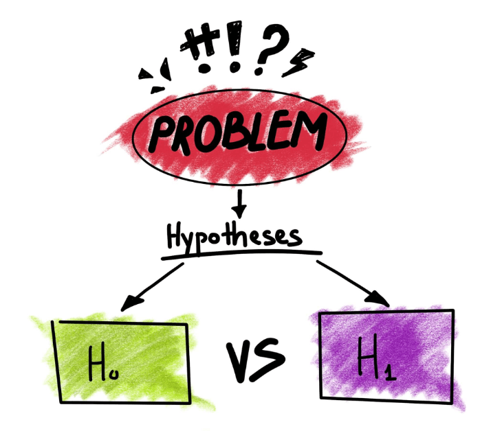
Hypothesis

A hypothesis is a conjecture or explanation which is based on little data that serves as the basis for further research. But, keeping that definition in mind let’s continue with a simple explanation.

Hypothesis is a proposition made on the basis for reasoning without any assumption of actual result that will be deduced from the proposition.

For references:

Let’s say, when we make an argument that if we sleep for 8 hours then we will get better marks rather than if we sleep less.

Hypothesis Testing

The word "hypothesis testing" refers to a statistical procedure. In Hypothesis Testing there is a testing of any assumption over a population parameter.

It is employed to judge how plausible the hypothesis is.

When it comes to the digital world, Hypothesis Testing is a machine learning based task which is generally done by python.

Purpose of Hypothesis Testing

It is a crucial step in statistics. Using sample data, a hypothesis test evaluates which of two statements about a population that are incompatible with one another is more strongly supported. A hypothesis test is what we allows us to state that a result is statistically significant.

Basis of Hypothesis:

Normalisation and Standard Normalisation are the foundation of a hypothesis.

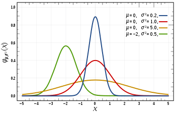
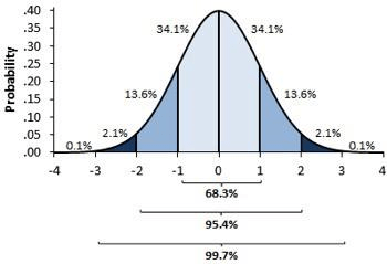
• Normal Distribution: If a variable's distribution resembles a normal curve i.e., a unique bell-shaped curve, then it is said to have a normal distribution or to have this property.  The normal curve, which is the graph of a normal distribution, possesses each of the qualities listed below.

• Standard Normal Distribution: The term "standard normal distribution" refers to a normal distribution with a mean of 0 and a standard deviation of 1.

Significant Parameters of Hypothesis Testing

The null hypothesis is a broad assertion or default stance in inferential statistics that there is no correlation between two measurable events or no link between groups.

In other words, it is a fundamental assumption or one based on an understanding of the problem or subject.

For instance, a corporation may produce 50 items every day, etc.

Alternative Hypothesis

In hypothesis testing, the alternative hypothesis is the theory that differs from the null hypothesis. Typically, it is assumed that the observations are the product of an actual impact (with some amount of chance variation superposed)

For instance, a corporation may not produce 50 items each day.

Level Of Significance

The fixed likelihood that the null hypothesis will be incorrectly eliminated when it is actually true is the degree of significance. The likelihood of type I mistake is defined as the degree of significance, and the researcher sets it based on the outcomes of the error. The assessment of statistical significance is called degree of significance. Whether the null hypothesis is thought to be accepted or rejected is specified. If the outcome is statistically significant, it should be possible to conclude that the null hypothesis is either incorrect or invalid.

It is impossible to accept or reject a hypothesis with 100% precision,so we choose a level of significance that is typically 5%.

This is typically indicated with the mathematical symbol alpha, which is typically 0.05 or 5%, meaning that you should have 95% confidence that your output will provide results that are comparable in each sample.

Type I error:

Despite the fact that the null hypothesis was correct, we reject it. Alpha is used to indicate a type I mistake. The alpha area is the portion of the normal curve that displays the important region in hypothesis testing.

Type II error

When the null hypothesis is accepted but is incorrect. The sign of a type II mistake is beta. The section of the normal curve that displays the acceptance region in a hypothesis test is referred to as the beta region.

One-tailed test

If just one side of the sample distribution has an area of rejection, the test of a statistical hypothesis is said to be one-tailed.

For instance, data science is being adopted by 80% of a college's 4000 students.

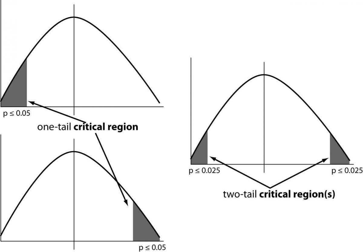
Two-tailed test

A two-sided critical area of a distribution is used in the two-tailed test to assess if a sample is more than or less than a specific range of values. If any of the key areas apply to the sample being tested, the alternative hypothesis will be used instead of the null hypothesis.

For instance, a school= 4,500 students, or data analyst = 83% of organisations embrace.

P Value

The likelihood of discovering the observed, or more extreme, outcomes when the null hypothesis (H 0) of a study question is true is known as the P value, or computed probability. The definition of what is considered to be "extreme" depends on how the hypothesis is being tested.

When your P value falls below the selected threshold of significance then the null hypothesis is rejected . It is agreed  that your sample contains solid evidence that the alternative hypothesis is true. It does not imply any  significant or important  difference i.e. : that it is prominently subjective while considering the real-world cases.

For reference:

Let’s take a case with a coin that you have and you don’t know that it is fair or it is tricky.

So let’s decide it with the NULL and Alternate Hypothesis.

H0=For Fair coin

H1=For Tricky coin and alpha=0.05

Let’s Workout for P-value

When we toss a coin for the first time if it gives Tail then P-value is =50%

When we toss the coin for the second time the if it gives the Tail again then the P-value is=25%

Then after trying for 6 consecutive times then P-value=1.5%

As we have set our significance to 95% that means that our error rate is 5% level.

We are beyond that level so our null hypothesis holds a good stand so we need to reject it.

Degree Of Freedom:

Degrees of freedom are the number of independent variables that can be estimated in a statistical analysis.

For better understanding of the hypothesis testing, let’s look on some widely use

Hypothesis testing type using python.

• T Test ( Student T test)
• Z Test
• ANOVA Test
• Chi-Square Test

T test

The t-test is a kind of inferential statistic that is used to assess if there is a significant difference between the means of two groups that could be connected by certain characteristics.

It is typically employed when data sets, such those obtained from tossing a coin 100 times and recorded as results, would follow a normal distribution and could have unknown variances.

The T test is a method for evaluating hypotheses that allows you to evaluate a population-applicable assumption.

There are Two Types of T-test:

1. One Sampled T-test
2. Two Sampled T-test

One Sampled T-test

Using the One Sample t Test, you may find out if the sample mean differs statistically from a real or hypothesised population mean. A parametric test is the One Sample t Test.

For reference:  You have to check whether the average age of the 10 ages taken is 30 or not.

Code:

from scipy.stats import ttest_1samp
import numpy as np
sammples_of_all_ages = np.genfromtxt("ages.csv")
print(sammples_of_all_ages)
data_mean = np.mean(sammples_of_all_ages)
print(data_mean)
tset, pval = ttest_1samp(sammples_of_all_ages, 30)
print("P-value",pval)
if pval < 0.05:    # alpha value is 0.05 or 5%
   print(" Null Hypothesis is being rejected")
else:
  print("Null Hypothesis is being accepted")

Output:

[30. 23. 45. 31. 34. 36. 42. 60. 23. 30.]
35.4
P-value 0.16158645446293013
Null Hypothesis is being accepted

Two Sampled Test

The Independent Samples t Test, also known as the 2-sample t-test, examines the means of two independent groups to see if there is statistical support for the notion that the related population means are statistically substantially different. It is  an  example of a parametric test.

Code:

from scipy.stats import ttest_ind
import numpy as np
first_Week= np.genfromtxt("week1.csv", delimiter=",")
second_Week= np.genfromtxt("week2.csv", delimiter=",")


print("Data of First Week :")
print(first_Week)
print("\nData of Second Week :")
print(second_Week)


mean_Of_First_Week = np.mean(first_Week)
mean_Of_Second_Week = np.mean(second_Week)


print("\nfirst_Week mean value:",mean_Of_First_Week)
print("second_Week mean value:",mean_Of_Second_Week)


std_Of_Fist_Week= np.std(first_Week)
std_Of_Second_Week = np.std(second_Week)


print("\nfirst_Week std value:",std_Of_Fist_Week)
print("second_Week std value:",std_Of_Second_Week)


ttest,pval = ttest_ind(first_Week,second_Week)
print("\np-value",pval)


if pval <0.05:
  print("\nREJECTING THE NULL HYPOTHESIS")
else:
  print("\nACCEPTING THE NULL HYPOTHESIS")

Output:

Data of First Week :
[1.2354 3.5685 5.8974 3.7894 6.8945 5.5685 5.6448 6.4752 7.7841 6.7846
 4.5684 6.4579 7.5461 8.9456 6.5489 4.5858 9.4563 8.1523 7.8945 2.5613
 1.5632 9.8945 7.5612 7.5647 8.8945]


Data of Second Week :
[1.2154 3.5455 7.8974 7.7894 6.8945 7.5685 2.6448 6.4752 5.7841 1.7846
 2.5684 5.4579 2.5461 4.9456 3.5489 2.5858 7.4563 6.1523 5.8945 3.5613
 2.5632 3.8945 5.5612 5.5647 6.8945]


first_Week mean value: 6.233504
second_Week mean value: 4.831784


first_Week std value: 2.306689087931878
second_Week std value: 2.0245040191968005


p-value 0.029934418917393343


REJECTING THE NULL HYPOTHESIS

Paired sampled t-test

The dependent sample t-test is another name for the paired sample t-test. It is a univariate test that looks for a meaningful distinction between two closely related variables. An instance of this would be taking a person's blood pressure before and after a certain therapy, condition, or time period.

H0 :- Refers to the difference between two sample is 0

H1:- Refers to the  difference between two sample is not 0

For Example:

We have taken blood pressure  tests , before and after a certain treatment of 120 people.

Code:

import pandas as pd
from scipy import stats


test_samples = pd.read_csv("blood.csv")
test_samples[['bp_before','bp_after']].describe()
ttest,pval = stats.ttest_rel(test_samples['bp_before'], test_samples['bp_after'])


print(pval)
if pval<0.05:
    print("REJECTING THE NULL HYPOTHESIS")
else:
    print("ACCEPTING THE NULL HYPOTHESIS")

Result:

0.0011297914644840823

REJECTING THE NULL HYPOTHESIS

Z-Test

The main purpose for using the Z-test is that it follow certain criteria in comparison to the T test which are given below:

• If it is feasible, sample sizes need to be comparable.
• Your data should be picked at random from a population in which each possible item has a fair probability of being chosen.
• You have a sample size of more than 30. If not, employ a t test.
• Data should be normally distributed.
• There should be no correlation between any two data points. To put it another way, two data points are unrelated or unaffected by one another.

For Example:-

We are again going to take the blood pressure test for Z Test (One Sample Test)

Code:

import pandas as pd
from scipy import stats
from statsmodels.stats import weightstats as stests
	
test_samples = pd.read_csv("blood.csv")
ztest ,pval = stests.ztest(test_samples['bp_before'], x2=None, value=156)
print(float(pval))


if pval<0.05:
    print("REJECTING THE NULL HYPOTHESIS")
else:
    print("ACCEPTING THE NULL HYPOTHESIS")

Output:

0.6651614730255063

ACCEPTING THE NULL HYPOTHESIS

We can do the two sample test for Z Test also

Two Sample Test

Similar to a t-test, we are comparing the sample means of two independent data sets to see whether they are equal.

H0 : 0 is the mean of two groups.

H1 : 0 is not the mean of two groups.

For Example:-

We taking the same blood pressure test for sake of convenience

Code:

import pandas as pd
from scipy import stats
from statsmodels.stats import weightstats as stests


test_samples = pd.read_csv("blood.csv")
ztest ,pval = stests.ztest(test_samples['bp_before'], x2=test_samples['bp_after'], value=0,alternative='two-sided')
print(float(pval))
if pval<0.05:
    print("REJECTING THE NULL HYPOTHESIS")
else:
    print("ACCEPTING THE NULL HYPOTHESIS")

Output:

0.002162306611369422

REJECTING THE NULL HYPOTHESIS

Anova Test(F-test)

The t-test is effective for comparing two groups, however there are situations when we wish to compare more than two groups at once. For instance, we would need to compare the means of each level or group in order to determine whether voter age varied depending on a categorical variable like race. We could do a separate t-test for each pair of groups, but doing so raises the possibility of false positive results. A statistical inference test that allows for simultaneous comparison of numerous groups is the analysis of variance, or ANOVA.

F=Variability between group/ Variability within group

Note:

The F-distribution does not have any negative values, unlike the z- and t-distributions, because the within- group variability is always positive as a result of squaring each deviation.

One Way F-test(Anova)

On the basis of their mean similarity and f-score of two or more groups, it  determines if they are similar or not.

Example:

Checking the similarity among three types of plants on the basis of their category and weight.

Csv  File data in a sheet format:

Sr no.	weight	group
1	4.17	ctrl
2	5.58	ctrl
3	5.18	ctrl
4	6.11	ctrl
5	4.5	ctrl
6	4.61	ctrl
7	5.17	ctrl
8	4.53	ctrl
9	5.33	ctrl
10	5.14	ctrl
11	4.81	trt1
12	4.17	trt1
13	4.41	trt1
14	3.59	trt1
15	5.87	trt1
16	3.83	trt1
17	6.03	trt1
18	4.89	trt1
19	4.32	trt1
20	4.69	trt1
21	6.31	trt2
22	5.12	trt2
23	5.54	trt2
24	5.5	trt2
25	5.37	trt2
26	5.29	trt2
27	4.92	trt2
28	6.15	trt2
29	5.8	trt2
30	5.26	trt2

Code:

import pandas as pd
from scipy import stats
from statsmodels.stats import weightstats as stests


df_anova = pd.read_csv('PlantGrowth.csv')
df_anova = df_anova[['weight','group']]


grps = pd.unique(df_anova.group.values)
d_data = {grp:df_anova['weight'][df_anova.group == grp] for grp in grps}
 
F, p = stats.f_oneway(d_data['ctrl'], d_data['trt1'], d_data['trt2'])


print("p-value for significance is: ", p)


if p<0.05:
    print("REJECTING THE NULL HYPOTHESIS")
else:
    print("ACCEPTING THE NULL HYPOTHESIS")

Output:

p-value for significance is:  0.0159099583256229

REJECTING THE NULL HYPOTHESIS

Two Way F-Test(Anova)

When we have two independent variables and two or more groups, we utilise the two-way F-test, which is an extension of the one-way F-test. The 2-way F-test cannot identify the dominating variable. Post-hoc testing must be carried out if individual significance needs to be verified.

Now let's examine the Grand mean crop yield (the mean crop yield without regard to any subgroup), the mean crop yield for each individual element, and the mean crop yield for all of the factors together.

Example with Code:

Yielding capacity of certain type of fertiles.

Csv  File data in a sheet format:

Fert	Water	Yield
A	High	27.4
A	High	33.6
A	High	29.8
A	High	35.2
A	High	33
B	High	34.8
B	High	27
B	High	30.2
B	High	30.8
B	High	26.4
A	Low	32
A	Low	32.2
A	Low	26
A	Low	33.4
A	Low	26.4
B	Low	26.8
B	Low	23.2
B	Low	29.4
B	Low	19.4
B	Low	23.8

Code:

import pandas as pd
import statsmodels.api as sm
from statsmodels.formula.api import ols
df_anova2 = pd.read_csv("https://raw.githubusercontent.com/Opensourcefordatascience/Data-sets/master/crop_yield.csv")
model = ols('Yield ~ C(Fert)*C(Water)', df_anova2).fit()
print(f"Overall model F({model.df_model: .0f},{model.df_resid: .0f}) = {model.fvalue: .3f}, p = {model.f_pvalue: .4f}")
res = sm.stats.anova_lm(model, typ= 2)
res

Output:

Overall model F( 3, 16) =  4.112, p =  0.0243

Chi-Square Test:

When there are two categorical variables from the same population, the test is used. It is used to decide if the two variables significantly associate with one another.

For instance, voters may be categorised in an election poll according to voting choice and gender (male or female) (Democrat, Republican, or Independent). To find out if gender affects voting choice, we might perform an independent chi-square test.

Example with code:

Which gender like shopping the most?

Csv File data in a sheet format:

Gender	Shopping?
Male	No
Female	Yes
Male	Yes
Female	Yes
Female	Yes
Male	Yes
Male	No
Female	No
Female	No

Code:

from re import T
import pandas as pd
from scipy import stats
from statsmodels.stats import weightstats as stests


df_chi_test= pd.read_csv("shop.csv")
table_Of_contingency=pd.crosstab(df_chi_test["Gender"],df_chi_test["Shopping?"])
print('contingency_table :-\n',table_Of_contingency)




#Values that are observed
values_Observed = table_Of_contingency.values
print("Observed Values :-\n",values_Observed)


b=stats.chi2_contingency(table_Of_contingency)
values_expected = b[3]
print("Expected Values :-\n",values_expected)


row_no=len(table_Of_contingency.iloc[0:2,0])
coloumn_no=len(table_Of_contingency.iloc[0,0:2])
ddof=(row_no-1)*(coloumn_no-1)
print("Degree of Freedom:-",ddof)


alpha = 0.05
from scipy.stats import chi2


chi_square_o=sum([(o-e)**2./e for o,e in zip(values_Observed,values_expected)])
chi_square_stats=chi_square_o[0]+chi_square_o[1]
print("chi-square statistic:-",chi_square_stats)
critical_value=chi2.ppf(q=1-alpha,df=ddof)
print('critical_value:',critical_value)


#p-value
p_value=1-chi2.cdf(x=chi_square_stats,df=ddof)
print('p-value \(level of marginal significance within a statistical hypothesis test\) :',p_value)
print('Level of Significance: ',alpha)
print('Degree of Freedom for hypothesis: ',ddof)
print('chi-square statistic for the hypothesis :',chi_square_stats)
print('critical_value of the hypothesis:',critical_value)
print('p-value \(level of marginal significance within a statistical hypothesis test\):',p_value)
if chi_square_stats>=critical_value:
    print("Reject H0,Two category variables are related to one another.")
else:
    print("Retain H0,Two category variables are not related to one another")
   
if p_value<=alpha:
    print("Reject H0,Two category variables are related to one another")
else:
    print("Retain H0,Two category variables are not related to one another")

Output:

contingency_table :-
 Shopping?  No  Yes
Gender
Female      2    3
Male        2    2
Observed Values :-
 [[2 3]
 [2 2]]
Expected Values :-
 [[2.22222222 2.77777778]
 [1.77777778 2.22222222]]
Degree of Freedom:- 1
chi-square statistic:- 0.09000000000000008
critical_value: 3.841458820694124
p-value \(level of marginal significance within a statistical hypothesis test\) : 0.7641771556220945
Level of Significance:  0.05
Degree of Freedom for hypothesis:  1
chi-square statistic for the hypothesis : 0.09000000000000008
critical_value of the hypothesis: 3.841458820694124
p-value \(level of marginal significance within a statistical hypothesis test\): 0.7641771556220945
Retain H0,Two category variables are not related to one another
Retain H0,Two category variables are not related to one another