Decision Tree Classification in Python

In this article, we will learn the implementation of the decision tree in Sklearn, which is nothing but the Scikit Learn library of python. First, we should learn what classification is.

What is Classification?

Classification is dividing the datasets into different categories or groups by adding the label. In another way, we can say that it is the technique of categorizing the observation into a different category.

We are taking the data, analyzing it, and based on some conditions, dividing it into various categories.

Why do We Classify it?

We classify it to perform productive analysis on it. Like when we get the mail, the Machine predicts whether it is said to be spam or not spam mail, and based on that prediction, it adds the irrelevant or spam mail to the respective folder.

In general, the classification algorithm handled questions like, is this data belong to the A category or B category? Is this a male, or is this female?

We will use this protection to check whether the transaction is genuine or not. Suppose we use a credit card in India because we had to fly to America; now, we will get a notification alert regarding my transaction if we use the credit card over there.

They would ask me to confirm the transaction. So, there is also a kind of predictive analysis as the Machine predicts something fishy in the transaction. Before 36 hours, we had done a transaction using the same credit card in India, and 24 hours later, the same credit card I used for the payment in America. To confirm it, it sends us a notification alert.

This is one of the use cases of classification. We can even use it to classify different items like fruits based on their color, size, and taste.

A well-trained machine using the classification algorithm can easily predict the class or type of fruit. Whenever new data is given to it, not just a fruit, it can be any item, it can be a car, or it can be a house, it can be a signboard or anything.

Types of Classification

There are several ways to perform the same task. A machine had to be trained first to predict whether a given person is a male or female. There are multiple ways to train the Machine, and you can choose one. There are many distinguishable techniques for predictive analysis, but the decision tree is the most call of them all is the decision tree.

As a part of the classification algorithm, we have:

1. Decision tree
2. Random forest
3. Naive Bayes
4. KNN algorithm
5. Logistic regression
6. Linear regression

Now, we will discuss the Decision Tree

Decision Tree

The decision tree is a graphical representation of all the possible solutions to a decision. The decisions which are made can be explained very easily. For example, here is a task which says should I go to a restaurant or should I buy Pasta. I am confused about that, so I will create a decision tree for it starting with the root node. Will first, we want to check whether I am hungry or not. If I am not hungry, then I go back to sleep. If I am hungry and I have 1000 rupees, I will decide to go to the restaurant, and If I am hungry and do not have 1000 rupees, then I will go and buy Pasta. So, this is about the decision tree.

What is a decision tree?

This decision tree is very easy to read and understand. It belongs to one of the few interpretable models where you can understand exactly why the classifier made that decision. For a given dataset, you cannot say that this algorithm performs better than that. It is like you cannot say that a decision tree is better than a bias or Naive bias performs better than a decision tree. It only depends on the dataset. We have to apply the hit and trial method with all the algorithms and then compare the result. The model that gives the best result is the model we can use for better accuracy for our data set.

" A decision tree is a graphical representation of all the possible solutions to a decision based on certain conditions."

Decision Tree Algorithm

As we discussed, the decision tree definition and we might wonder why this is called a decision tree, because it starts with a root and then branches off to several solutions, just like a tree, even the tree starts from a root. It starts growing its branches once it gets bigger and bigger. Similarly, a decision tree has a root that keeps on growing with increasing decisions and conditions.

We would now check with a real-life scenario. Whenever I dial the toll-free number of my company, it redirects to the intelligent computerized assistant like press 1 for English or press 2 for Hindi, press 3 for Telugu and so on. Suppose now you select 1; it again redirects to a certain set of questions like as same above. So, this keeps on repeating until you get to the right person.

Consider an example of a decision tree that has created a decision tree: "Should I accept a new job offer?" For this, we have a root node named a "salary of at least 50,000 rupees." If it is YES, the commute is more than 1 hour or not; if it is YES, I will decline the offer. I will accept the job offer if it is less than 1 hour. Further, I will check whether the company is offering free coffee; if the company is not offering free coffee, I will decline the offer, and if it offers free coffee, I will happily accept it. So, this is the only example of a decision tree.

Now, let us consider a sample dataset we will use to explain the decision tree. Each row in this data set is an example; the first two columns provide features or attributes that describe the data, and the last column gives the label or the class we want to predict. And if we want to modify this data by adding additional features and examples, our program will work the same way. It is straightforward except for one thing: it is not perfectly separable. In the second and fifth examples, they have the same features but different labels; both have yellow as their color and a diameter of three, but the labels are mango and lemon.

Let us see how a decision tree handles this case. To build a tree will use a decision tree algorithm called "Carter". So, this carter algorithm stands for classification and regression tree algorithm.

Terminology of a Decision Tree

So let us start with the root node. The root node is a base node of a tree; the entire tree starts from a root node. In other words, it is the first node of a tree, representing the entire population or samples of this population, that is further segregated or divided into two or more homogeneous sets.

Next, we will discuss the leaf node. The leaf node is the one when you reach the end of the tree. That is when we cannot further segregate it to another level.

Now we will discuss splitting. It divides our root node or node into different sub-parts based on some condition.

Now comes the branch or sub-tree. This branch or sub-tree formed when we split the tree. Suppose when we split a root node, it gets divided into two branches or two sub-trees.

Next is the concept of Pruning. It is just the opposite of splitting, and we are just removing the sub-node of a decision tree.

Next is the parent or child node. As we know that root node is always a parent node, and all other associated nodes are known as child nodes. All the top nodes belong to a parent node all the bottom nodes derived from a top node are a child node. The node producing a different node is a child node, and the node producing it is a parent.

We will discuss further the decision tree.

A decision tree is a type of supervised learning algorithm that is used for both classification and regression problems. This algorithm will use training data to create rules representing a tree structure. Like a tree, it consists of the root, internal, and leaf nodes.

How does a Tree Decide Where to Split?

Before we split a tree, we should know some terminologies. The first is the GINI INDEX. So, Gini Index is the measure of Impurity (or purity) used in building the decision tree in CART ALGORITHM.

Information Gain

This information gain is the decrease in entropy after a dataset is split based on an attribute. Constructing a decision tree involves finding attributes that return the highest information gain. So, we will be selecting the node that would give us the highest information gain.

Reduction in Variance

Reducing variance is an algorithm for continuous target variables (regression problems). The split with lower variance is selected as the criteria to split the population.

Variance is how much our data varies. So, if our data is less impure or is purer, then, in that case, the variation would be less as all the data is almost similar. It is also a way of splitting a tree, and then spread with lower variance is selected as a criterion to split the population.

Chi-Square

It is an algorithm to determine the statistical significance of the differences between sub-nodes and the parent node.

First, we know how to decide on the best attribute. For this, we need to calculate information to gain the attribute with the highest information gain is considered the best. To define the correct definition for information gain, we would first know about the term "Entropy". In this definition, it helps to calculate the information gained.

Entropy

Entropy is just a metric that measures the Impurity of something; in other words, we can say that it is the first step before you solve the problem for the decision tree.

Let us now understand what the term is called Impurity.

Suppose we have a basket full of apples and another bowl full of some label that says Apple. Now, if you are asked to pick one item from each basket and ball, then the probability of getting the apple and the correct label is 1, so in this case, we can say that Impurity is '0'.

Now, if there are four different fruits in the basket and 4 different labels on the ball, then the probability of matching the fruit to the label is not 1. It is something less than that. It could be possible that when I pick a banana from the basket and randomly pick the label from the ball, it says a cherry; any random permutation and the combination can be possible. So, in this case, I would say that impurities are non-zero.

Entropy

It is the measure of Impurity. It is just a metric that measures the Impurity to the first step to solving a decision tree problem.From the graph given below, we can say that as the probability is '0.' or '1', that is either they are highly impure or it is highly pure; then, in that case, the value of entropy is '0', and when the probability is 0.5 then the value of entropy is maximum. Impurity is the degree of randomness; that is, how random a data is?

We have a mathematical formula for entropy that is shown below:

Entropy(s) = -P(Yes) log2 P(Yes) - P(no) log2 P(no)

Where we derive that,

S is the total sample space

P(Yes) is the probability of YES

If number of YES = number of NO i.e., P(S) = 0.5

1. Entropy(s) = 1

If it contains all YES or all NO i.e., P(S) = 1 or 0

2. (s) = 0

When P(Yes) = P(No) = 0.5 i.e., YES+NO = Total Sample(S)

Here, we have an equal number of Yes equal to NO's probability.

When we put the values in the 1st formula, we get

E(S) = 0.5 log2 0.5 - 0.5 log2 0.5

E(S) = 0.5(log2 0.5 - log2 0.5)

E(S) = 1

From above we get the total sample space as "ONE".

In the second case, we would consider

E(S) = -P(Yes) log2 P(Yes)

When P(Yes) = 1 i.e., YES = Total Sample(S)

E(S) = 1 log1 base 2

Above, the value of log 1 = 0.

Similarly in the case NO we get the entropy of total sample space is "0". Below shows you an example.

E(S) = -P(No) log2 P(No)

when P(No) = 1 i.e., NO= Total Sample(S)

E(S) = 1 log2 1

E(S) = 0

Here entropy of total sample space is "0".

What is Information Gain?

It measures the reduction in entropy and decides which attribute should be selected as the decision node.

If "S" is our total collection,

Information Gain = Entropy(S) - [(Weighted Avg) * Entropy (each feature)]

Let us build our own decision tree.

So, let us manually build a decision tree for our data set, consisting of 14 instances, of which we have 9 YES and 5 NO. So, we have a formula for entropy.

We have 9, YES, and so the total probability of YES is 9/14

The total probability of NO is 5/14.

When we calculate the value of entropy, we get,

E(S) = -P(Yes)log2 P(Yes)-P(No) log2 P(No)

E(S) = -(9/14) *log2 9/14-(5/14) * log2 5/14

E(S) =0.41+0.53 --> 0.94

So, the value of entropy as 0.94.

Out of those 5 nodes, we will get confused about which node is the root node. Based on this, we would be creating the entire tree.

We must calculate the entropy, and Information gained for all the nodes.

Starting with "Outlook" has three different parameters that are sunny, overcast and rainy. Firstly, check how many YES and NO are there.

Then, we will calculate the entropy for each feature. Here we are calculating for "outlook".

E (Outlook = Sunny) = -2/5 log2 2/5

E (Outlook = Overcast) = -1 log2 1 - 0 log 2 0 = 0

E (Outlook = Sunny) = -3/5 log2 3/5 - 2/5 log2 2/5 =0.971

Information from outlook,

I(Outlook) = 5/14*0.971 + 4/14*0+5/14*0.971=0.693

Information gained from outlook is

Gain (Outlook) = E(S)-I(Outlook)

0.94-0.693=0.247

Like this, we can calculate each feature from the above table.

Importing Libraries

We should import the libraries that are initially required, such as NumPy, pandas, seaborn, and matplotlib. pyplot.

import numpy as np
import pandas as pd
import seaborn as sns
import matplotlib.pyplot as plt
%Matplotlib inline

Importing the dataset

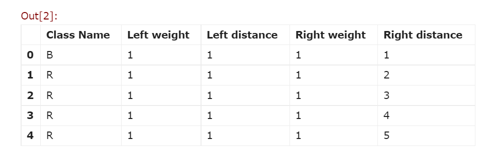
Here we will import the dataset from a CSV file to the pandas' data frames.

col = [ 'Class Name', 'Left weight', 'Left distance', 'Right weight', 'Right distance']
df = pd.read_csv('balance-scale.data', names=col, sep=',')
df.head ()  

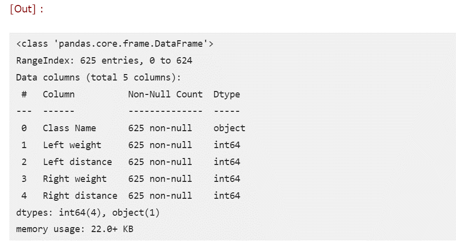
When we want dataset information, we must use a function called "df.info". From the above output, we can see that it already has 625 records and 5 fields.

df.info ()

Output

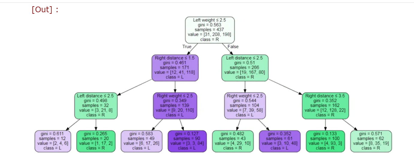
Plotting a Decision Tree

We can also plot the decision tree as a tree structure by using a library called Graphviz library. Then, we can pass several parameters such as the classifier model, target values, and our data's features name.

target = list(df['Class Name']. unique ())
feature names = list (Columns)

And also, we should write another program for plotting a decision tree.

from sklearn import tree
import graphviz
dot_data = tree.export_graphviz(clf_model,
out_file=None, 
feature_names=feature_names,  
class_names=target,  
                      filled=True, rounded=True,  
special_characters=True)  
graph = graphviz.Source(dot_data)  
graph

Output

Also, we can get the tree by textual representation by using the export_tree function from the sklearn library.

When to Stop Splitting?

1. The stopping condition is met
2. Possible to split until 1 leaf for each observation (100% accuracy)
3. Overfitting problem
4. Set constraints on tree size
5. Tree pruning

Advantages of Decision Tree

1. Easy to Understand: Decision tree output is very easy to understand, even for people from a non-analytical background.
2. Useful in Data Exploration: A decision tree is one of the fastest ways to identify the most significant variables and the relation between two or more variables.
3. Handle Outliers: It is not influenced by outliers and missing values to a fair degree.
4. The data type is not a constraint: It can handle both numerical and categorical variables.
5. Non-Parametric Method: The decision tree is considered to be a non-parametric method. Decision trees have no assumptions about space distribution and the classifier structure.

Disadvantages of Decision Tree

1. Over Fitting: Overfitting is one of the most practical difficulties for decision tree models. This problem gets solved by setting constraints on model parameters and pruning.
2. Limitation for Continuous Variables: While working with continuous numerical variables, the decision tree losses information when it discretizes variables in different categories.

Some points on the decision tree

• A decision tree is very simple to understand and interpret.
• Incorporates, academics, social events etc., plays a very important role.
• With other decision techniques can also be used.
• Addition can also do in the decision tree with a new scenario.
• Information or data is needed and can include expert opinions and preferences. 
• Normalization of data does not require in the decision tree.
• Decision tree causes instability if there are any data or information changes.
• Calculations become difficult; particularly, it means values are uncertain and if many outcomes are linked.