Python Data Structures

Python Data Structures: Python is a programming language used worldwide for various fields such as building dynamic websites, artificial intelligence and many more. However, there is data that plays a very significant role in making all of this programming possible, which means how data should be stored effectively, and the access to it must be appropriate. So, the main problem is – How do we accomplish this? To solve this problem, Data Structures are introduced.

Thus, we will be discussing Python's Data Structures in detail throughout the following section.

Understanding the Data Structures

Data Structures are the method of organizing and managing the data which allow the user to store the collected data, relate them and perform different operations. There are various types of data structures defined to allow the computer engineers and data scientists to focus easily on the significant picture of solving bigger problems rather than getting lost in data reports and access facts.

Abstract Data Type in Data Structures

As discussed in the previous section, the data structures help users mainly focus on the main picture rather than getting lost in the facts. This process is also known as Data Abstraction.

Thus, the data structures are an application of ADT (abbreviated for Abstract Data Types). This application or implementation needs a physical view of data with the help of some collection of basic data types and programming constructs.

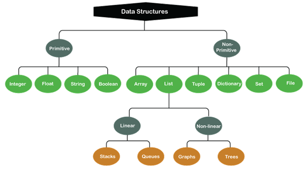
Usually, in computer science, these data structures can be classified into two distinct categories: the first category is primitive data structures, and the other is related to non-primitive data structures. The simplest forms of data representation are the former, whereas the more advanced and complex are the latter. These consist of primitive data structures within more complex and advanced data structures for special purposes.

The Primitive Data Structures

The predefined and basic method of storing data by the system are known as Primitive Data structures. They also have a predefined set of operations for performing them on the data. These Data structures work as the building blocks to manipulate data and store pure and simple data values. Four primitive variable types are defined in Python, and these are as follows:

1. Integers

2. Strings

3. Boolean

4. Float

Let's discuss them in brief in the next sections.

Integers

We can utilize the integer data type to represent the numeric data. More specifically, it is used to represent the whole numbers from negative infinity to infinity, for example, 52, 23, 0, or -8

String

Strings are collections of alphabets, words or many other characters. We can create the string data type in Python by including an order of characters within a pair of single or double-quotes. For example: 'tutorial', "example", etc.

There are several operations we can perform with strings. For example, we can concatenate two or more strings together by applying the + operation on them, as shown below:

>>> x = 'tutorial'
>>> y = 'example'
>>> x + ' & ' + y
'tutorial & example'

We can repeat a string for a certain number of times by using the * operation on them, as shown below:

>>> x = 'tutorial'
>>> x * 2
'tutorialtutorial'

We can also select the parts of strings by slicing the strings. Here's an illustration is given below:

>>> # This is Range Slicing
>>> a1 = x[4:]
>>> print(a1)
rial
>>> # This is Slicing
>>> a2 = y[1] + y[4]
>>> print(a2)
xp

Note – We can also use alphanumeric characters as the strings; however, the + operation is still be used for concatenating strings.

>>> a = '5'
>>> b = '6'
>>> a + b
'56'

There are various built-in methods functions available in Python for manipulating strings. Some common string manipulation methods are capitalizing certain words in a paragraph, replacing a substring, and finding a string's position within another string. Some of these are illustrated below:

• For capitalizing strings

>>> str.capitalize('tutorial')
'Tutorial'

• For checking whether a string contains only digits or not.

>>> a = '13'
>>> b = 'example'
>>> a.isdigit()
True
>>> b.isdigit()
False

• For retrieving the length of a string in characters, including the spaces between the words:

>>> a = 'tutorial 4 u'
>>> b = 'example'
>>> len(a)
12
>>> len(b)
7

• For replacing the parts of strings with other strings

>>> a.replace('tutorial', b)
'example 4 u'

• For finding substrings in other strings. This method is used to return the position or lowest index within the string at which the substring is found:

>>> a = 'tutorial'
>>> b = 'tutor'
>>> a.find(b)
0

As we can see that the substring 'tutor' is found at the beginning of 'tutorial'. In the output, we refer to the position with 'tutorial' at which we find that substring which is in this can is 0.

Here's another example based on this.

>>> a = 'This is a tutorial'
>>> b = 'tutor'
>>> a.find(b)
10

In this case, our substring 'tutor' is found at the 10th index within 'This is a tutorial'. And we need to remember that we have to start counting from 0 and include the spaces afterward.

Boolean

The Boolean is a built-in data type used to return the values: True and False, which can often be interchangeable with the integers, 0 or 1. These are pretty useful in comparison and conditional expressions. Let's see some examples based on Booleans.

>>> a = 6
>>> b = 8
>>> a == b
False
 
>>> b > a
True
 
>>> a = 3
>>> b = 4
>>> c = (a == b) # comparison expression (Estimates to false)
>>> if c: # conditional on true/false value of ‘c’
...     print("Hello World!")
... else: print("Goodbye World!")
...
Goodbye World!

Float

The Float is also a built-in data type that stands for 'floating point number'. These can be used for representing rational numbers that usually ends with a decimal figure, for example, 3.14, 2.05 or 12.34

Let's see some examples based on Float.

>>> a = 3.0    # these are some examples
>>> b = 6.0    # of float

We can perform various operations on integers and floats. Some of them are shown below:

• We can simply add two or more integers or float numbers.

>>> print(a + b)
9.0

• We can also perform subtraction with integers and float numbers.

>>> print(b - a)
3.0

• We can also perform multiplication with integers and float numbers.

>>> print(a * b)
18.0

• We can also perform an operation to return the quotient.

>>> print(b / a)
2.0

• We can also perform an operation to return the remainder.

>>> print(b % a)
0.0

• We can also perform an operation to print the absolute value of an integer or a float value.

>>> print(abs(a))
3.0

• Many other operations can be performed with integers and float numbers, such as assigning power to a variable.

>>> print(b ** a)
216.0

Note: Python is a dynamically typed language, where the data type is stored mutable as an object. Thus, we do not have to explicitly state the type of data or variable.

The Data Type Conversion

Let's take an example,  sometimes we find ourselves stuck converting an integer to a float or vice versa while working on someone else's code or maybe find ourselves using an integer when we need Float in the code. So, in such cases, we can convert the data type of variables.

First of all, there is a built-in type() function defined in Python to check an object's type. Here's an example illustrating the usage of this function:

>>> x = 3.0
>>> type(x)
<class 'float'>

Now, let’s understand the concept behind the conversion of data types or, in other terms, Typecasting. Typecasting means to convert the type of an object from one data type to another. The data type conversions are broadly classified into two categories: Implicit (also termed as coercion) and Explicit (also mentioned as casting)

Implicit Data Type Conversion

Implicit Data Type Conversion is an automatic data conversion where the compiler handles the operations for the user. Let's have a look at some example shown below:

>>> a = 5.0          # a float
>>> b = 3           # an integer
>>> c = a * b       # multiplying ‘a’ and ‘b’
>>> type(c)          # checking the type of ‘c’
<class 'float'>

As we can see in the above example, we did not explicitly convert the data type of 'b' to carry out the float value multiplication. The compiler did the operation implicitly by itself.

Explicit Data Type Conversion

The Explicit Data Type Conversion is a user-defined data conversion where a user explicitly informs the compiler to change certain objects' data type. Let's have a look at an example shown below:

>>> a = 4
>>> b = 'Rick and Morty: Season '
>>> latest_season = b + a
Traceback (most recent call last):
  File "<stdin>", line 1, in <module>
TypeError: unsupported operand type(s) for +: 'int' and 'str'

As we can see, the above snippet of code has given us an error saying unsupported operand type(s). This is because the compiler does not understand that we are attempting to perform a concatenation of two variables due to the mixed data types. One variable is an integer, and the other is a string that we are trying to concatenate together. Thus, giving an error for an obvious divergence.

Thus, firstly, we need to convert the integer to a string to solve the above problem and perform the concatenation.

Note: It might not be possible to change the type of a variable or data into another every time. There are few built-in functions used for data conversion and can be useful for the above problem. Some of them are: int(), str(), and float()

>>> a = 4
>>> b = 'Rick and Morty: Season '
>>> latest_season = (b) + str(a)
>>> print(latest_season)
Rick and Morty: Season 4

The Non-Primitive Data Structures

Non-Primitive data Structures act as the complex components of the data structures family. Instead of storing a value, these data structures have a collection of values in different formats.

In the conventional world of computer science, non-primitive data structures are further classified into multiple categories:

• Arrays
• Lists
• Files

Array

First of all, arrays are the data structures with a complex method to collect the basic data types in Python. All the entries must be of the same data type in an array. However, this data structure is not much popular in Python as in other programming languages, like C++ or Java.

Usually, when people talk about the arrays in Python, they are indicating to the lists. But the arrays are quite different from the lists, and we will be discussing this sooner. Arrays have a more efficient method to store a certain type of list. Though, the list should have the elements of the same data type.

Arrays are represented by the array module in Python and are required to be imported before initializing and taking them in action. In an array, the elements stored are constricted to their data type. The data type is specified while creating the array and represented with the help of a type code. This type code is a single character representation of the data types; for example, ‘I’ is the type code for integer, whereas ‘f’ represents the float and many more. Let’s see an example based on the array.

>>> import array as ar
>>> x = ar.array("I",[2,4,6])
>>> type(x)
<class 'array.array'>

Some commonly used type codes are listed in the following table:

Type Code	Python Type	C Type	Min bytes
i	int	signed int	2
I	int	unsigned int	2
f	float	float	4
g	float	double	8
h	int	signed short	2
H	int	unsigned short	2
l	int	signed long	4
L	int	unsigned long	4
b	int	signed char	1
B	int	unsigned char	1
u	Unicode	Py_UNICODE	2

The array module's various methods and functionalities are easily accessible in Python Array documentation.

Lists

Lists are the data structures used to store a collection of heterogeneous items in Python. Lists are mutable, which indicates that their content can be changed by modifying their identity. The lists can be represented by the square brackets: [ ], which helps hold the elements, divided by a comma ‘,’. These are built-in Python data structures, and there is no need to invoke them discretely. Let’s see some examples based on the lists.

>>> a = []          # an empty list
>>> type(a)
<class 'list'>

>>> a1 = [1, 2, 3, 4, 5]
>>> type(a1)
<class 'list'>

>>> a2 = list([3, 'banana', 4])
>>> type(a2)
<class 'list'>

>>> print(a2[1])
banana
>>> a2[1] = 'mango'
>>> print(a2)
[3, 'mango', 4]

Note: As we can see in the above example with a1, the list holds homogeneous items, which also implies that the list can also be used to store homogeneous items. This also satisfies the storage functionality of an array. It is okay to unless we are applying some particular operations to the collection.

There are various methods available in python for manipulating and working with lists. For example, adding a new item in a list, removing some items from a list, sorting or reversing a list and many more. Following are the some of the common list manipulations.

• Adding 10 to the my_list list using the append() method. However, this number will be added to the end of the list by default.

>>> my_list = [12, 56, 34, 78, 123, 90, 901, 789, 456]

>>> my_list.append(10)              # adding 10 to the list

>>> print(my_list)

[12, 56, 34, 78, 123, 90, 901, 789, 456, 10]

Inserting 10 at the position or index 0 in the my_list list using the insert() method.

>>> my_list.insert(0, 10)  # inserting 10 at the 0th index

>>> print(my_list)

[10, 12, 56, 34, 78, 123, 90, 901, 789, 456, 10]

Removing the first occurrence of ‘e’ from the ur_list list using the remove() method.

>>> ur_list = ['e', 'x', 'a', 'm', 'p', 'l', 'e']

>>> ur_list.remove('e')    # removing the first 

                             # occurrence of e

>>> print(ur_list)

['x', 'a', 'm', 'p', 'l', 'e']

Removing the item at the index -3 from the ur_list list using the pop() method.

>>> ur_list.pop(-3)        # removing the item

                            # from the specified index

'p'

>>> print(ur_list)

['x', 'a', 'm', 'l', 'e']

Sorting the items of the my_list list using the sort() method.

>>> my_list.sort()         # in-place sorting

>>> print(my_list)

[10, 10, 12, 34, 56, 78, 90, 123, 456, 789, 901]

Reversing the items of the my_list list using the reverse() method.

>>> list.reverse(my_list)
>>> print(my_list)
[901, 789, 456, 123, 90, 78, 56, 34, 12, 10, 10]

Usually, the list data structure can be further classified into two sub-categories: Linear Data Structures and Non-Linear Data Structures. The Linear data structures consist of Stacks and Queues, whereas the Non-Linear data structures consist of Graphs and Trees. The structures and concepts of these data structures are relatively complex. However, their similarity to real-world models let them being used extensively. We will be having a glimpse of these topics in the following sections.

Note: The data items are ordered consecutively or, in simple terms, linearly in a Linear data structure. All of these data items can be navigated consecutively one after another in a single run. In contrast, the items of data are not organized consecutively in Non-linear data structures. That implies that a non-linear data structure could be connected to multiple elements reflecting a special relationship among these data items. Moreover, in a non-linear data structure, the data items may not be navigated during a single run.

Stacks

A container of objects where objects are removed and inserted according to the LIFO (Last-In-First-Out) principle is known as Stack. Let’s take an example where there is a stack of plates at a dinner party. These plates are always removed from or added to the top of the pile. The same concept is opted in computer science to evaluate expressions and parse syntax, scheduling algorithms or routines and many more.

In Python, the stacks can be implemented with the help of lists. Some operations are also used in a stack known as push and pop. The Push operation is used to add elements to a stack, whereas the Pop operation is used to delete or remove an element.

# (Bottom) 1 < 2 < 3 < 4 < 5 < 6 (Top)
>>> my_stack = [1, 2, 3, 4, 5, 6]
>>> my_stack.append(7)   # (B) = 1 < 2 < 3 < 4 < 5 < 6 < 7 = (T)
>>> print(my_stack)
[1, 2, 3, 4, 5, 6, 7]
>>> my_stack.pop()        # removing the top element (7)
7
>>> print(my_stack)
[1, 2, 3, 4, 5, 6]        # (B) = 1 < 2 < 3 < 4 < 5 < 6 = (T)
>>> my_stack.pop()        # removing the top element (6) again
6
>>> print(my_stack)
[1, 2, 3, 4, 5]            # (B) = 1 < 2 < 3 < 4 < 5 = (T)

Queue

A container of objects where objects are removed and inserted according to the FIFO (First-In-First-Out) concept is known as Queue. Let’s take an example of a line at a ticket counter for a ride in an amusement park. The people are treated according to their arrival sequence. And hence the individual who reaches first is also the first to leave. There can be various kinds of Queues.

A queue is not efficiently be implemented with the use of lists. This is because the append() and pop() methods are not fast, and incur movement cost to memory. Moreover, the deletion from the beginning and insertion at the end of a list is not pretty fast as it needs a shift in the element positions.

Graphs

In Mathematics and Computer Science, the networks consist of vertices (also called nodes) is known as a graph. These nodes may or may not be connected. The path or the line that helps in connecting two nodes is known as an edge. The graph is said to be directed if the edge has a particular flow direction, where the direction edge is known as an arc. At the same time, the graph is said to be undirected if no directions are specified.

This concept may sound pretty abstract and can become more complex when we start digging in depth. But in Data Science, graphs are a significant concept and often practiced to solve real-world problems. Various sectors depend on the graph and its theory principles such as social networks, maps, molecular studies in biology and chemistry, recommender system and many more.

To get started, let’s have a look at a simple graph implementation with the help of a Python Dictionary:

my_graph = {
            "a" : ["b", "c"],
            "b" : ["c", "d"],
            "c" : ["d", "e"],
            "d" : ["e", "a"],
            "e" : ["a", "b"]
            }
def def_edges(my_graph):
    my_edges = []
    for my_vertices in my_graph:
        for neighbor in my_graph[my_vertices]:
            my_edges.append((my_vertices, neighbor))
    return my_edges
print(def_edges(my_graph))

The Output of above snippet of code should look as follows:

[('a', 'b'), ('a', 'c'), ('b', 'c'), ('b', 'd'), ('c', 'd'), ('c', 'e'), ('d', 'e'), ('d', 'a'), ('e', 'a'), ('e', 'b')]

There is a lot of cool stuff that we can do with graphs. For example, we can find the shortest path between two nodes, or we can determine cycles in the graph and many more.

Trees

A tree is a living organism with its roots deep down in the ground and the branches holding the leaves in the actual world. These trees branches spread out in a slightly organized system. Trees also play a significant role in computer science, describing the data in an organized manner. However, the root is on top and the branches spread towards the bottom, and the whole tree is illustrated inverted when compared to the actual tree.

The Tree data structure starts with the root on the top, following the other nodes (also known as branches) spreading downwards with the final nodes (also known as leaves) attached to each branch. We can also visualize that each branch is a smaller tree itself. The root at the top is often known as a parent. At the same time, the nodes at the end of each branch are referred to as its children. Moreover, the nodes attached to the same parent are called siblings. Thus, we can also conclude the wholesome as a family tree.

The Tree data structure supports defining real-world situations and is utilized in almost every sector. Whether in the gaming industry designing XML parsers or the PDF designing principle, all are based on tree data structures. Moreover, ‘Decision Tree based learning’ has also increased a large research area in Data Science. Many well-known methods such as bagging, boosting and many more are use the tree concept for generating an analytical model. Even games like chess are built on the concept of tree analyzing the possible moves and apply heuristics for deciding on an ideal move.

The tree data structure can be implemented using and combining the multiple data structures discussed so far. Let’s see an example to understand this very concept.

class Tree:

    def __init__(self, info, left = None, right = None):

        self.info = info

        self.left  = left

        self.right = right

    def __str__(self):

        return (str(self.info) + ', First Factor: ' + str(self.left) + ', Second Factor: ' + str(self.right))

my_tree = Tree(60, Tree(15, 3, 5), Tree(4, 2, 2))

print("Factor Tree of 60")

print(my_tree)

The Output for above snippet of code should appear as shown below:

Factor Tree of 60

60, First Factor: 15, First Factor: 3, Second Factor: 5, Second Factor: 4, First Factor: 2, Second Factor: 2

We have discussed about the data structures like arrays and lists. Let’s explore some different variety of data collection methods in Python. Although these data structure might be differ from the traditional data structures stated in computer science, they are worth eloquent especially with respect to Python programming language:

• Tuples
• Dictionary
• Sets

Tuples

Tuples are one of the standard sequence data structures. However, tuples differ from lists as tuples are immutable, which implies that they cannot be deleted, added or edited once they are defined. Tuples play a very significant role in scenarios where we have to pass the control to someone else but not allow them to manipulate data in the collection and many more. Let’s have a look at the implementation of tuples in the following example:

>>> tuple_a = 2, 4, 6, 8, 10
>>> tuple_b = ('p', 'q', 'r', 's', 't')
>>> tuple_a[0]
2
>>> tuple_b[2]
'r'
>>> tuple_a[0] = 3      # cannot change the value inside a tuple

Traceback (most recent call last):
  File "", line 1, in
TypeError: 'tuple' object does not support item assignment

Dictionary

Implementing a data structure like a dictionary becomes necessary when talking about something similar to a telephone directory. We have not discussed any such data structures before that are suitable for a telephone directory.

So, most of us might be thinking, what is the basic idea behind Dictionary? To understand the problem, let’s take the example of a telephone directory. As we know, the telephone directory consists of so many contact numbers for their contact names. This is when a data structure like a dictionary becomes handy. Dictionaries are comprised of key-value pairs. The key is used to identify the item, whereas the value is holding the item's value. Thus, the telephone directory has a key (contact name) and the value (contact number) assigned to that key.

>>> dict_a = {'Apple': 1, 'Banana': 2, 'Mango': 3, 'Orange': 4}
>>> del dict_a['Orange']
>>> dict_a
{'Apple': 1, 'Banana': 2, 'Mango': 3}
>>> dict_a['Banana']     # Prints the value stored with the key
2

There are various built-in functions available for dictionaries. Let’s try them in following examples:

>>> len(dict_a)
3

 >>> dict_a.keys()
dict_keys(['Apple', 'Banana', 'Mango'])

 >>> dict_a.values()
dict_values([1, 2, 3])

Sets

The Set data structure is used to represent a collection of diverse (unique) objects. The Sets play a significant role in creating lists holding unique values only in the dataset. It is an unordered collection but a mutable one. This property of sets helps while working with a huge dataset. Here are some examples based on sets and their functionalities.

>>> my_set = set('TUTORIAL')
>>> ur_set = set('EXAMPLE')
>>> print(my_set)
{'A', 'T', 'R', 'L', 'I', 'O', 'U'}
>>> print(ur_set)
{'X', 'A', 'P', 'M', 'L', 'E'}
>>> print(my_set - ur_set)         # All the elements of my_set
                                     # but not in ur_set
{'T', 'R', 'I', 'O', 'U'}
>>> print(my_set | ur_set)         # All the unique elements of
                                     # my_set and ur_set
{'X', 'A', 'T', 'P', 'R', 'L', 'I', 'O', 'M', 'E', 'U'}
>>> print(my_set & ur_set)         # Element common in both
                                     # my_set and ur_set
{'A', 'L'}

Files

Files are a part of traditional data structures in Python. In the Data Science industry, where big data appears to be usual, a programming language without the ability to store and recover formerly stored data or information would barely be convenient. We still need to make use of all the information sitting in the file across the database. Let’s have a glimpse of how this process works.

Python provides a similar background to other programming languages for writing the code to read and write files with a lot easier way to handle. Some of the fundamental methods and functions that allows one user to interact with files using Python are shown below:

• The read() method is used to read entire files;
• The open() method is used to open files in the system where filename is the name of the file to be opened;
• The write() method is used to write a string to a file and also returns the number of characters written;
• The readline() method is used to read one line at a time; and
• The close() method is used to close the opened file.

# File Mode (Second Argument): 'w'(write), 'r'(read), 'r+'(both reading and writing), 'a'(appending)
# Opening a file
f = open('file_name.txt', 'r')

 # Reading an entire file
f.read()

 # Reading one line at a time
f.readline()

 # Writing the string to the file, returning the number of characters written
f.write('Add this line.')
 
# Closing the file
f.close()

The second argument of the open() method is the file mode. It helps in specifying the mode of the file whether the user wants to write (w), read (r), append (a) or both read and write (r+).